Algorithm principles and implementation with YOLOv5¶

0 Introduction¶

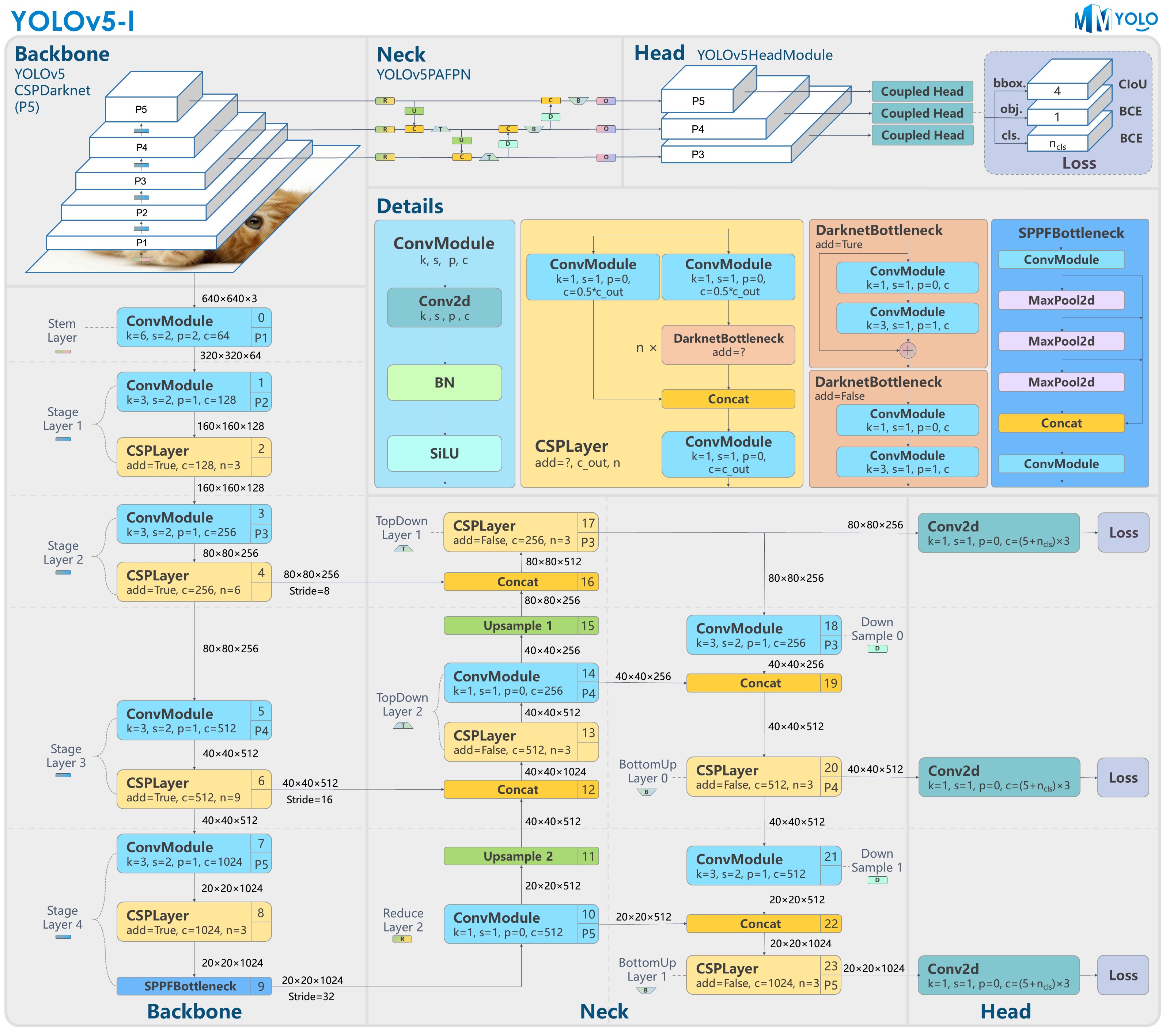Figure 1: YOLOv5-l-P5 model structure

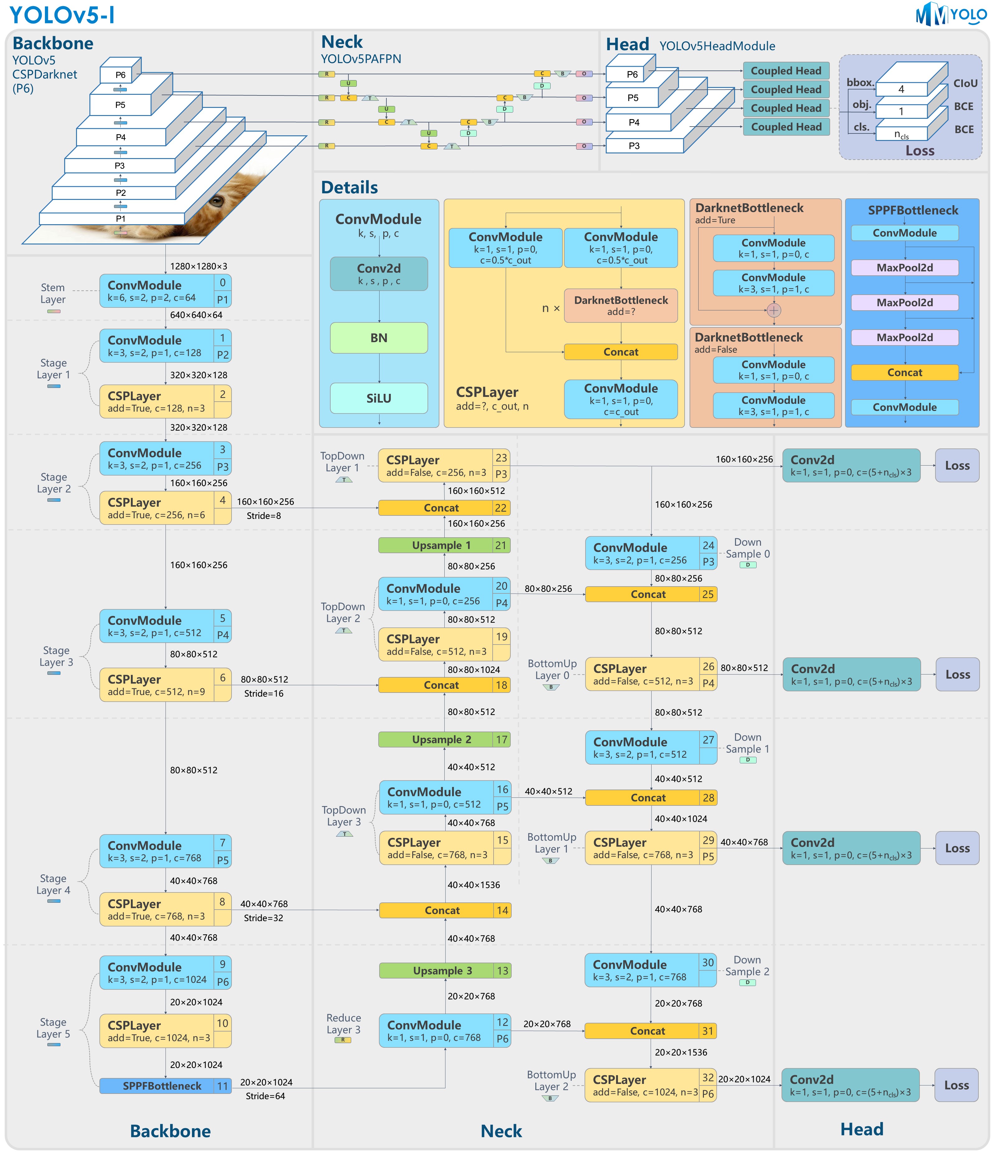Figure 2: YOLOv5-l-P6 model structure

RangeKing@github provides the graph above. Thanks, RangeKing!

YOLOv5 is an open-source object detection algorithm for real-time industrial applications which has received extensive attention. The reason for the explosion of YOLOv5 is not simply due to its excellent performance. It is more about the overall utility and robustness of its library. In short, the main features of YOLOv5 are:

Friendly and perfect deployment supports
Fast training speed: the training time in the case of 300 epochs is similar to most of the one-stage and two-stage algorithms under 12 epochs, such as RetinaNet, ATSS, and Faster R-CNN.
Abundant optimization for corner cases: YOLOv5 has implemented many optimizations. The functions and documentation are richer as well.

Figures 1 and 2 show that the main differences between the P5 and P6 versions of YOLOv5 are the network structure and the image input resolution. Other differences, such as the number of anchors and loss weights, can be found in the configuration file. This article will start with the principle of the YOLOv5 algorithm and then focus on analyzing the implementation in MMYOLO. The follow-up part includes the guide and speed benchmark of YOLOv5.

Hint

Unless specified, the P5 model is described by default in this documentation.

We hope this article becomes your core document to start and master YOLOv5. Since YOLOv5 is still constantly updated, we will also keep updating this document. So please always catch up with the latest version.

MMYOLO implementation configuration: https://github.com/open-mmlab/mmyolo/blob/main/configs/yolov5/

YOLOv5 official repository: https://github.com/ultralytics/yolov5

1 v6.1 algorithm principle and MMYOLO implementation analysis¶

YOLOv5 official release: https://github.com/ultralytics/yolov5/releases/tag/v6.1

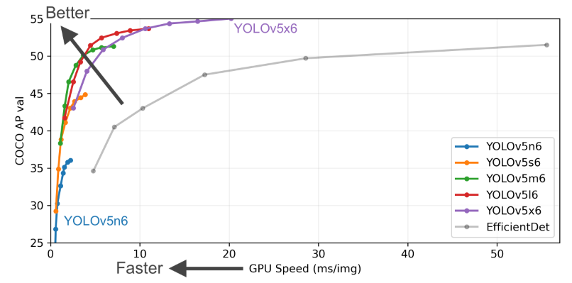
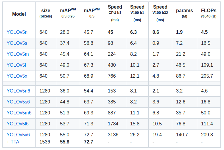
The performance is shown in the table above. YOLOv5 has two models with different scales. P6 is larger with a 1280x1280 input size, whereas P5 is the model used more often. This article focuses on the structure of the P5 model.

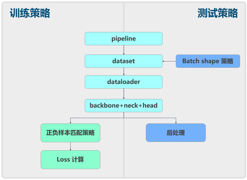
Usually, we divide the object detection algorithm into different parts, such as data augmentation, model structure, loss calculation, etc. It is the same as YOLOv5:

Now we will briefly analyze the principle and our specific implementation in MMYOLO.

1.1 Data augmentation¶

Many data augmentation methods are used in YOLOv5, including:

Mosaic
RandomAffine
MixUp
Image blur and other transformations using Albu
HSV color space enhancement
Random horizontal flips

The mosaic probability is set to 1, so it will always be triggered. MixUp is not used for the small and nano models, and the probability is 0.1 for other l/m/x series models. As small models have limited capabilities, we generally do not use strong data augmentations like MixUp.

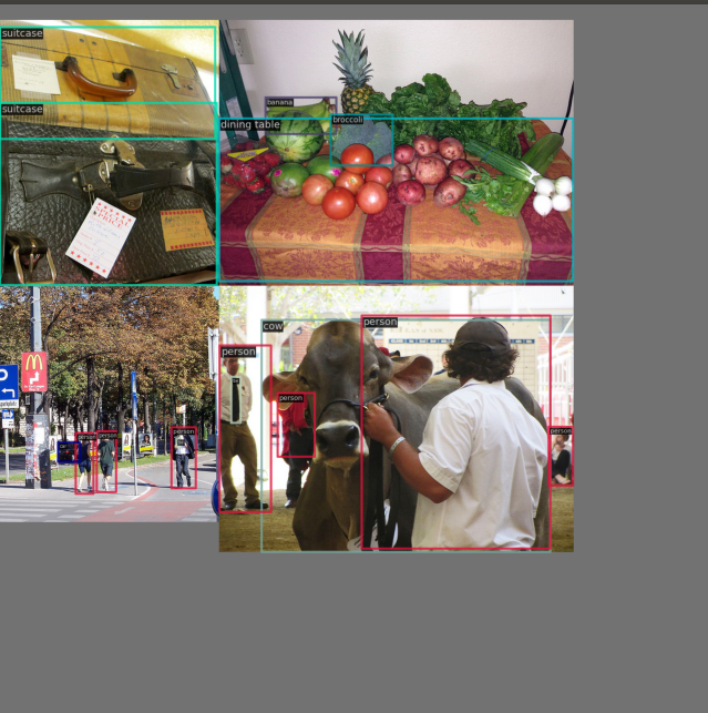
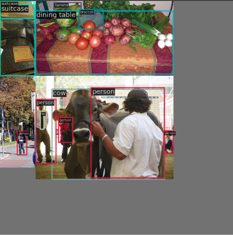
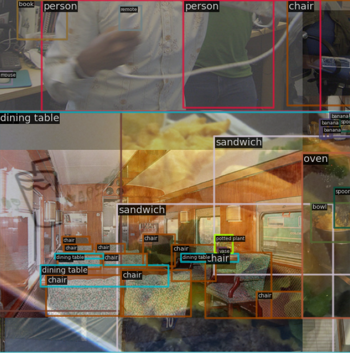
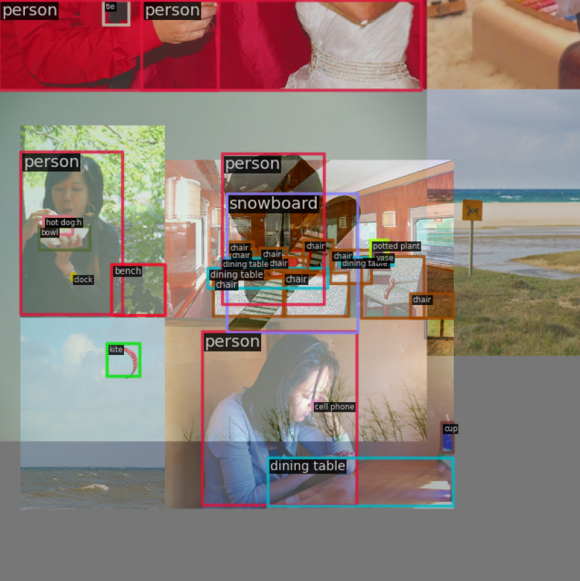
The following picture demonstrates the Mosaic + RandomAffine + MixUp process.

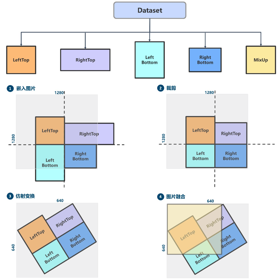
1.1.1 Mosaic¶

Mosaic is a hybrid data augmentation method requiring four images to be stitched together, which is equivalent to increasing the training batch size.

We can summarize the process as:

Randomly generates coordinates of the intersection point of the four spliced images.
Randomly select the indexes of the other three images and read the corresponding annotations.
Resizes each image to the specified size by maintaining its aspect ratio.
Calculate the position of each image in the output image according to the top, bottom, left, and right rule. You also need to calculate the crop coordinates because the image may be out of bounds.
Uses the crop coordinates to crop the scaled image and paste it to the position calculated. The rest of the places will be pad with 114 pixels.
Process the label of each image accordingly.

Note: since four images are stitched together, the output image area will be enlarged four times (from 640x640 to 1280x1280). Therefore, to revert to 640x640, you must add a RandomAffine transformation. Otherwise, the image area will always be four times larger.

1.1.2 RandomAffine¶

RandomAffine has two purposes:

Performs a stochastic geometric affine transformation to the image.
Reduces the size of the image generated by Mosaic back to 640x640.

RandomAffine includes geometric augmentations such as translation, rotation, scaling, misalignment, etc. Since Mosaic and RandomAffine are strong augmentations, they will introduce considerable noise. Therefore, the enhanced annotations need to be processed. The rules are

The width and height of the enhanced gt bbox should be larger than wh_thr;
The ratio of the area of gt bbox after and before the enhancement should be greater than ar_thr to prevent it from changing too much.
The maximum aspect ratio should be smaller than area_thr to prevent it from changing too much.

Object detection algorithms will rarely use this augmentation method as the annotation box becomes larger after the rotation, resulting in inaccuracy.

1.1.3 MixUp¶

MixUp, similar to Mosaic, is also a hybrid image augmentation. It randomly selects another image and mixes the two images together. There are various ways to do this, and the typical approach is to either stitch the label together directly or mix the label using alpha method. The original author’s approach is straightforward: the label is directly stitched, and the images are mixed by distributional sampling.

Note: In YOLOv5’s implementation of MixUP, the other random image must be processed by Mosaic+RandomAffine before the mixing process. This may not be the same as implementations in other open-source libraries.

1.1.4 Image blur and other augmentations¶

The rest of the augmentations are:

Image blur and other transformations using Albu
HSV color space enhancement
Random horizontal flips

The Albu library has been packaged in MMDetection so users can directly use all Albu’s methods through simple configurations. As a very ordinary and common processing method, HSV will not be further introduced now.

1.1.5 The implementations in MMYOLO¶

While conventional single-image augmentations such as random flip are relatively easy to implement, hybrid data augmentations like Mosaic are more complicated. Therefore, in MMDetection’s reimplementation of YOLOX, a dataset wrapper called MultiImageMixDataset was introduced. The process is as follows:

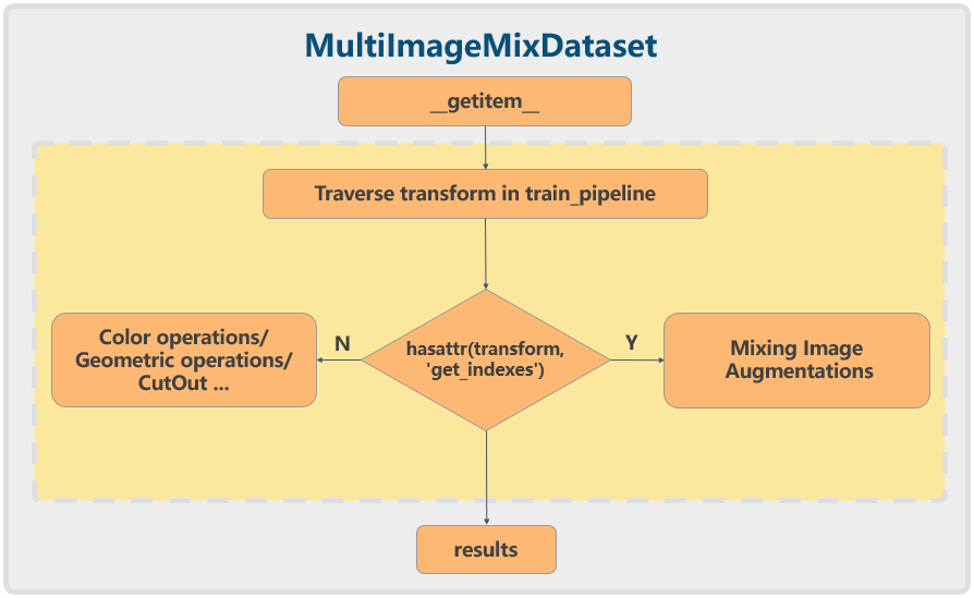
For hybrid data augmentations such as Mosaic, you need to implement an additional get_indexes method to retrieve the index information of other images and then perform the enhancement. Take the YOLOX implementation in MMDetection as an example. The configuration file is like this:

train_pipeline = [
    dict(type='Mosaic', img_scale=img_scale, pad_val=114.0),
    dict(
        type='RandomAffine',
        scaling_ratio_range=(0.1, 2),
        border=(-img_scale[0] // 2, -img_scale[1] // 2)),
    dict(
        type='MixUp',
        img_scale=img_scale,
        ratio_range=(0.8, 1.6),
        pad_val=114.0),
    ...
]

train_dataset = dict(
    # use MultiImageMixDataset wrapper to support mosaic and mixup
    type='MultiImageMixDataset',
    dataset=dict(
        type='CocoDataset',
        pipeline=[
            dict(type='LoadImageFromFile'),
            dict(type='LoadAnnotations', with_bbox=True)
        ]),
    pipeline=train_pipeline)

MultiImageMixDataset passes in a data augmentation method, including Mosaic and RandomAffine. CocoDataset also adds a pipeline to load the images and the annotations. This way, it is possible to quickly achieve a hybrid data augmentation method.

However, the above implementation has one drawback: For users unfamiliar with MMDetection, they often forget that Mosaic must be used with MultiImageMixDataset. Otherwise, it will return an error. Plus, this approach increases the complexity and difficulty of understanding.

To solve this problem, we have simplified it further in MMYOLO. By making the dataset object directly accessible to the pipeline, the implementation and the use of hybrid data augmentations can be the same as random flipping.

The configuration of YOLOX in MMYOLO is written as follows:

pre_transform = [
    dict(type='LoadImageFromFile'),
    dict(type='LoadAnnotations', with_bbox=True)
]

train_pipeline = [
    *pre_transform,
    dict(
        type='Mosaic',
        img_scale=img_scale,
        pad_val=114.0,
        pre_transform=pre_transform),
    dict(
        type='mmdet.RandomAffine',
        scaling_ratio_range=(0.1, 2),
        border=(-img_scale[0] // 2, -img_scale[1] // 2)),
    dict(
        type='YOLOXMixUp',
        img_scale=img_scale,
        ratio_range=(0.8, 1.6),
        pad_val=114.0,
        pre_transform=pre_transform),
    ...
]

This eliminates the need for the MultiImageMixDataset and makes it much easier to use and understand.

Back to the YOLOv5 configuration, since the other randomly selected image in the MixUp also needs to be enhanced by Mosaic+RandomAffine before it can be used, the YOLOv5-m data enhancement configuration is as follows.

pre_transform = [
    dict(type='LoadImageFromFile'),
    dict(type='LoadAnnotations', with_bbox=True)
]

mosaic_transform= [
    dict(
        type='Mosaic',
        img_scale=img_scale,
        pad_val=114.0,
        pre_transform=pre_transform),
    dict(
        type='YOLOv5RandomAffine',
        max_rotate_degree=0.0,
        max_shear_degree=0.0,
        scaling_ratio_range=(0.1, 1.9),  # scale = 0.9
        border=(-img_scale[0] // 2, -img_scale[1] // 2),
        border_val=(114, 114, 114))
]

train_pipeline = [
    *pre_transform,
    *mosaic_transform,
    dict(
        type='YOLOv5MixUp',
        prob=0.1,
        pre_transform=[
            *pre_transform,
            *mosaic_transform
        ]),
    ...
]

1.2 Network structure¶

This section was written by RangeKing@github. Thanks a lot!

The YOLOv5 network structure is the standard CSPDarknet + PAFPN + non-decoupled Head.

The size of the YOLOv5 network structure is determined by the deepen_factor and widen_factor parameters. deepen_factor controls the depth of the network structure, that is, the number of stacks of DarknetBottleneck modules in CSPLayer. widen_factor controls the width of the network structure, that is, the number of channels of the module output feature map. Take YOLOv5-l as an example. Its deepen_factor = widen_factor = 1.0. the overall structure is shown in the graph above.

The upper part of the figure is an overview of the model; the lower part is the specific network structure, in which the modules are marked with numbers in serial, which is convenient for users to correspond to the configuration files of the YOLOv5 official repository. The middle part is the detailed composition of each sub-module.

If you want to use netron to visualize the details of the network structure, open the ONNX file format exported by MMDeploy in netron.

Hint

The shapes of the feature map in Section 1.2 are (B, C, H, W) by default.

1.2.1 Backbone¶

CSPDarknet in MMYOLO inherits from BaseBackbone. The overall structure is similar to ResNet with a total of 5 layers of design, including one Stem Layer and four Stage Layer:

Stem Layer is a ConvModule whose kernel size is 6x6. It is more efficient than the Focus module used before v6.1.
Except for the last Stage Layer, each Stage Layer consists of one ConvModule and one CSPLayer, as shown in the Details part in the graph above. ConvModule is a 3x3 Conv2d + BatchNorm + SiLU activation function module. CSPLayer is the C3 module in the official YOLOv5 repository, consisting of three ConvModule + n DarknetBottleneck with residual connections.
The last Stage Layer adds an SPPF module at the end. The SPPF module is to serialize the input through multiple 5x5 MaxPool2d layers, which has the same effect as the SPP module but is faster.
The P5 model passes the corresponding results from the second to the fourth Stage Layer to the Neck structure and extracts three output feature maps. Take a 640x640 input image as an example. The output features are (B, 256, 80, 80), (B,512,40,40), and (B,1024,20,20). The corresponding stride is 8/16/32.
The P6 model passes the corresponding results from the second to the fifth Stage Layer to the Neck structure and extracts three output feature maps. Take a 1280x1280 input image as an example. The output features are (B, 256, 160, 160), (B,512,80,80), (B,768,40,40), and (B,1024,20,20). The corresponding stride is 8/16/32/64.

1.2.2 Neck¶

There is no Neck part in the official YOLOv5. However, to facilitate users to correspond to other object detection networks easier, we split the Head of the official repository into PAFPN and Head.

Based on the BaseYOLONeck structure, YOLOv5’s Neck also follows the same build process. However, for non-existed modules, we use nn.Identity instead.

The feature maps output by the Neck module is the same as the Backbone. The P5 model is (B,256,80,80), (B,512,40,40) and (B,1024,20,20); the P6 model is (B,256,160,160), (B,512,80,80), (B,768,40,40) and (B,1024,20,20).

1.2.3 Head¶

The Head structure of YOLOv5 is the same as YOLOv3, which is a non-decoupled Head. The Head module includes three convolution modules that do not share weights. They are used only for input feature map transformation.

The PAFPN outputs three feature maps of different scales, whose shapes are (B,256,80,80), (B,512,40,40), and (B,1024,20,20) accordingly.

Since YOLOv5 has a non-decoupled output, that is, classification and bbox detection results are all in different channels of the same convolution module. Taking the COCO dataset as an example:

When the input of P5 model is 640x640 resolution, the output shapes of the Head module are (B, 3x(4+1+80),80,80), (B, 3x(4+1+80),40,40) and (B, 3x(4+1+80),20,20).
When the input of P6 model is 1280x1280 resolution, the output shapes of the Head module are (B, 3x(4+1+80),160,160), (B, 3x(4+1+80),80,80), (B, 3x(4+1+80),40,40) and (B, 3x(4+1+80),20,20).

3 represents three anchors, 4 represents the bbox prediction branch, 1 represents the obj prediction branch, and 80 represents the class prediction branch of the COCO dataset.

1.3 Positive and negative sample assignment strategy¶

The core of the positive and negative sample assignment strategy is to determine which positions in all positions of the predicted feature map should be positive or negative and even which samples will be ignored.

This is one of the most significant components of the object detection algorithm because a good strategy can improve the algorithm’s performance.

The assignment strategy of YOLOv5 can be briefly summarized as calculating the shape-matching rate between anchor and gt_bbox. Plus, the cross-neighborhood grid is also introduced to get more positive samples.

It consists of the following two main steps:

For any output layer, instead of the commonly used strategy based on Max IoU matching, YOLOv5 switched to comparing the shape matching ratio. First, the GT Bbox and the anchor of the current layer are used to calculate the aspect ratio. If the ratio is greater than the threshold, the GT Bbox and Anchor are considered not matched. Then the current GT Bbox is temporarily discarded, and the predicted position in the grid of this GT Bbox in the current layer is regarded as a negative sample.
For the remaining GT Bboxes (the matched GT Bboxes), YOLOv5 calculates which grid they fall in. Using the rounding rule to find the nearest two grids and considering all three grids as a group that is responsible for predicting the GT Bbox. The number of positive samples has increased by at least three times compared to the previous YOLO series algorithms.

Now we will explain each part of the assignment strategy in detail. Some descriptions and illustrations are directly or indirectly referenced from the official repo.

1.3.1 Anchor settings¶

YOLOv5 is an anchor-based object detection algorithm. Similar to YOLOv3, the anchor sizes are still obtained by clustering. However, the difference compared with YOLOv3 is that instead of clustering based on IoU, YOLOv5 switched to using the aspect ratio on the width and height (shape-match based method).

While training on customized data, user can use the tool in MMYOLO to analyze and get the appropriate anchor sizes of the dataset.

python tools/analysis_tools/optimize_anchors.py ${CONFIG} --algorithm v5-k-means
 --input-shape ${INPUT_SHAPE [WIDTH HEIGHT]} --output-dir ${OUTPUT_DIR}

Then modify the default anchor size setting in the config file:

anchors = [[(10, 13), (16, 30), (33, 23)], [(30, 61), (62, 45), (59, 119)],
           [(116, 90), (156, 198), (373, 326)]]

1.3.2 Bbox encoding and decoding process¶

The predicted bounding box will transform based on the pre-set anchors in anchor-based algorithms. Then, the transformation amount is predicted, known as the GT Bbox encoding process. Finally, the Pred Bbox decoding needs to be performed after the prediction to restore the bboxes to the original scale, known as the Pred Bbox decoding process.

In YOLOv3, the bbox regression formula is:

\[\begin{split}b_x=\sigma(t_x)+c_x \\ b_y=\sigma(t_y)+c_y \\ b_w=a_w\cdot e^{t_w} \\ b_h=a_h\cdot e^{t_h} \\\end{split}\]

In the above formula，

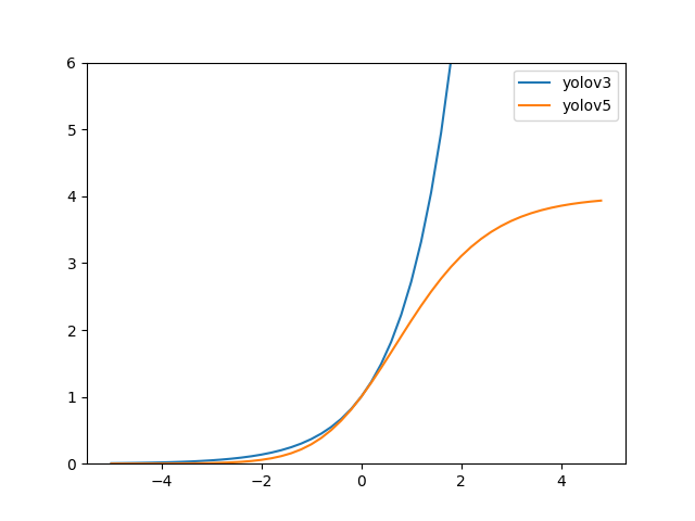
\[\begin{split}a_w represents the width of the anchor \\ c_x represents the coordinate of the grid \\ \sigma represents the Sigmoid function.\end{split}\]

However, the regression formula in YOLOv5 is：

\[\begin{split}b_x=(2\cdot\sigma(t_x)-0.5)+c_x \\ b_y=(2\cdot\sigma(t_y)-0.5)+c_y \\ b_w=a_w\cdot(2\cdot\sigma(t_w))^2 \\ b_h=a_h\cdot(2\cdot\sigma(t_h))^2\end{split}\]

Two main changes are:

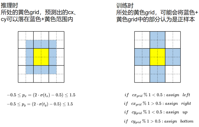
adjusted the range of the center point coordinate from (0, 1) to (-0.5, 1.5);
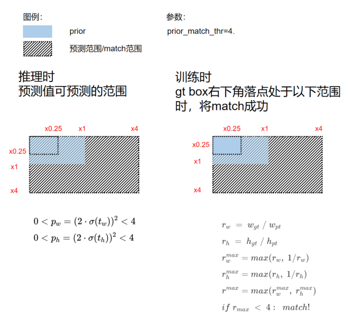
adjusted the width and height from

\[(0，+\infty)\]

to

\[(0，4a_{wh})\]

The changes have the two benefits:

It will be better to predict zero and one with the changed center point range, which makes the bbox coordinate regression more accurate.

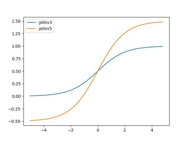
exp(x) in the width and height regression formula is unbounded, which may cause the gradient out of control and make the training stage unstable. The revised width-height regression in YOLOv5 optimizes this problem.

1.3.3 Assignment strategy¶

Note: in MMYOLO, we call anchor as prior for both anchor-based and anchor-free networks.

Positive sample assignment consists of the following two steps:

(1) Scale comparison

Compare the scale of the WH in the GT BBox and the WH in the Prior:

\[\begin{split}r_w = w\_{gt} / w\_{pt} \\ r_h = h\_{gt} / h\_{pt} \\ r_w^{max}=max(r_w, 1/r_w) \\ r_h^{max}=max(r_h, 1/r_h) \\ r^{max}=max(r_w^{max}, r_h^{max}) \\ if\ \ r_{max} < prior\_match\_thr: match!\end{split}\]

Taking the assignment process of the GT Bbox and the Prior of the P3 feature map as the example:

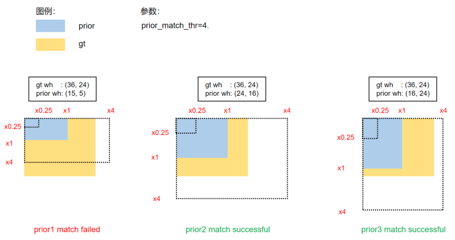
The reason why Prior 1 fails to match the GT Bbox is because:

\[h\_{gt}\ /\ h\_{prior}\ =\ 4.8\ >\ prior\_match\_thr\]

(2) Assign corresponded positive samples to the matched GT BBox in step 1

We still use the example in the previous step.

The value of (cx, cy, w, h) of the GT BBox is (26, 37, 36, 24), and the WH value of the Prior is [(15, 5), (24, 16), (16, 24)]. In the P3 feature map, the stride is eight. Prior 2 and prior 3 are matched.

The detailed process can be described as:

(2.1) Map the center point coordinates of the GT Bbox to the grid of P3.

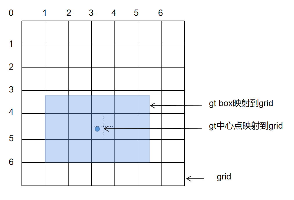
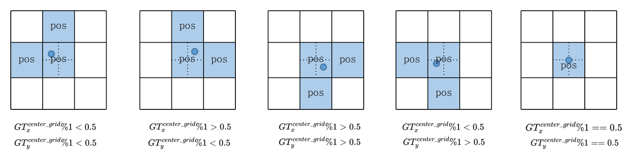
\[\begin{split}GT_x^{center_grid}=26/8=3.25 \\ GT_y^{center_grid}=37/8=4.625\end{split}\]

(2.2) Divide the grid where the center point of GT Bbox locates into four quadrants. Since the center point falls in the lower left quadrant, the left and lower grids of the object will also be considered positive samples.

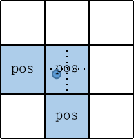
The following picture shows the distribution of positive samples when the center point falls to different positions:

So what improvements does the Assign method bring to YOLOv5?

One GT Bbox can match multiple Priors.
When a GT Bbox matches a Prior, at most three positive samples can be assigned.
These strategies can moderately alleviate the problem of unbalanced positive and negative samples, which is very common in object detection algorithms.

The regression method in YOLOv5 corresponds to the Assign method:

Center point regression:

WH regression:

1.4 Loss design¶

YOLOv5 contains a total of three Loss, which are:

Classes loss: BCE loss
Objectness loss: BCE loss
Location loss: CIoU loss

These three losses are aggregated according to a certain proportion:

\[Loss=\lambda_1L_{cls}+\lambda_2L_{obj}+\lambda_3L_{loc}\]

The Objectness loss corresponding to the P3, P4, and P5 layers are added according to different weights. The default setting is

obj_level_weights=[4., 1., 0.4]

\[L_{obj}=4.0\cdot L_{obj}^{small}+1.0\cdot L_{obj}^{medium}+0.4\cdot L_{obj}^{large}\]

In the reimplementation, we found a certain gap between the CIoU used in YOLOv5 and the latest official CIoU, which is reflected in the calculation of the alpha parameter.

In the official version:

Reference: https://github.com/Zzh-tju/CIoU/blob/master/layers/modules/multibox_loss.py#L53-L55

alpha = (ious > 0.5).float() * v / (1 - ious + v)

In YOLOv5’s version:

alpha = v / (v - ious + (1 + eps))

This is an interesting detail, and we need to test the accuracy gap caused by different alpha calculation methods in our follow-up development.

1.5 Optimization and training strategies¶

YOLOv5 has very fine-grained control over the parameter groups of each optimizer, which briefly includes the following sections.

1.5.1 Optimizer grouping¶

The optimization parameters are divided into three groups: Conv/Bias/BN. In the WarmUp stage, different groups use different lr and momentum update curves. At the same time, the iter-based update strategy is adopted in the WarmUp stage, and it becomes an epoch-based update strategy in the non-WarmUp stage, which is quite tricky.

In MMYOLO, the YOLOv5OptimizerConstructor optimizer constructor is used to implement optimizer parameter grouping. The role of an optimizer constructor is to control the initialization process of some special parameter groups finely so that it can meet the needs well.

Different parameter groups use different scheduling curve functions through YOLOv5ParamSchedulerHook.

1.5.2 weight decay parameter auto-adaptation¶

The author adopts different weight decay strategies for different batch sizes, specifically:

When the training batch size does not exceed 64, weight decay remains unchanged.
When the training batch size exceeds 64, weight decay will be linearly scaled according to the total batch size.

MMYOLO also implements through the YOLOv5OptimizerConstructor.

1.5.3 Gradient accumulation¶

To maximize the performance under different batch sizes, the author sets the gradient accumulation function automatically when the total batch size is less than 64.

The training process is similar to most YOLO, including the following strategies:

Not using pre-trained weights.
There is no multi-scale training strategy, and cudnn.benchmark can be turned on to accelerate training further.
The EMA strategy is used to smooth the model.
Automatic mixed-precision training with AMP by default.

What needs to be reminded is that the official YOLOv5 repository uses single-card v100 training for the small model with a bs is 128. However, m/l/x models are trained with different numbers of multi-cards. This training strategy is not relatively standard, For this reason, eight cards are used in MMYOLO, and each card sets the bs to 16. At the same time, in order to avoid performance differences, SyncBN is turned on during training.

1.6 Inference and post-processing¶

The YOLOv5 post-processing is very similar to YOLOv3. In fact, all post-processing stages of the YOLO series are similar.

1.6.1 Core parameters¶

multi_label

For multi-category prediction, you need to consider whether it is a multi-label case or not. Multi-label case predicts probabilities of more than one category at one location. As YOLOv5 uses sigmoid, it is possible that one object may have two different predictions. It is good to evaluate mAP, but not good to use. Therefore, multi_label is set to True during the evaluation and changed to False for inferencing and practical usage.

score_thr and nms_thr

The score_thr threshold is used for the score of each category, and the detection boxes with a score below the threshold are treated as background. nms_thr is used for nms process. During the evaluation, score_thr can be set very low, which improves the recall and the mAP. However, it is meaningless for practical usage and leads to a very slow inference performance. For this reason, different thresholds are set in the testing and inference phases.

nms_pre and max_per_img

nms_pre is the maximum number of frames to be preserved before NMS, which is used to prevent slowdown caused by too many input frames during the NMS process. max_per_img is the final maximum number of frames to be reserved, usually set to 300.

Take the COCO dataset as an example. It has 80 classes, and the input size is 640x640.

The inference and post-processing include:

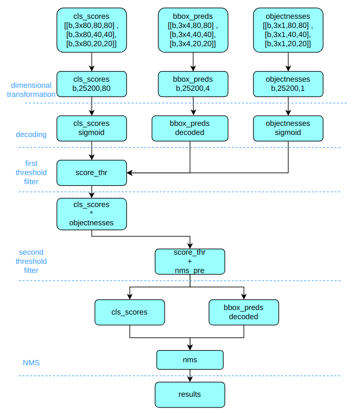
(1) Dimensional transformation

YOLOv5 outputs three feature maps. Each feature map is scaled at 80x80, 40x40, and 20x20. As three anchors are at each position, the output feature map channel is 3x(5+80)=255. YOLOv5 uses a non-decoupled Head, while most other algorithms use decoupled Head. Therefore, to unify the post-processing logic, we decouple YOLOv5’s Head into the category prediction branch, the bbox prediction branch, and the obj prediction branch.

The three scales of category prediction, bbox prediction, and obj prediction are stitched together and dimensionally transformed. For subsequent processing, the original channel dimensions are replaced at the end, and the shapes of the category prediction branch, bbox prediction branch, and obj prediction branch are (b, 3x80x80+3x40x40+3x20x20, 80)=(b,25200,80), (b,25200,4), and (b,25200,1), respectively.

(2) Decoding to the original graph scale

The classification branch and obj branch need to be computed with the sigmoid function, while the bbox prediction branch needs to be decoded and reduced to the original image in xyxy format.

(3) First filtering

Iterate through each graph in the batch, and then use score_thr to threshold filter the category prediction scores to remove the prediction results below score_thr.

(4) Second filtering

Multiply the obj prediction scores and the filtered category prediction scores, and then still use score_thr for threshold filtering. It is also necessary to consider multi_label and nms_pre in this process to ensure that the number of detected boxes after filtering is no more than nms_pre.

(5) Rescale to original size and NMS

Based on the pre-processing process, restore the remaining detection frames to the original graph scale before the network output and perform NMS. The final output detection frame cannot be more than max_per_img.

1.6.2 batch shape strategy¶

To speed up the inference process on the validation set, the authors propose the batch shape strategy, whose principle is to ensure that the images within the same batch have the least number of pad pixels in the batch inference process and do not require all the images in the batch to have the same scale throughout the validation process.

It first sorts images according to their aspect ratio of the entire test or validation set, and then forms a batch of the sorted images based on the settings. At the same time, the batch shape of the current batch is calculated to prevent too many pad pixels. We focus on padding with the original aspect ratio but not padding the image to a perfect square.

        image_shapes = []
        for data_info in data_list:
            image_shapes.append((data_info['width'], data_info['height']))

        image_shapes = np.array(image_shapes, dtype=np.float64)

        n = len(image_shapes)  # number of images
        batch_index = np.floor(np.arange(n) / self.batch_size).astype(
            np.int64)  # batch index
        number_of_batches = batch_index[-1] + 1  # number of batches

        aspect_ratio = image_shapes[:, 1] / image_shapes[:, 0]  # aspect ratio
        irect = aspect_ratio.argsort()

        data_list = [data_list[i] for i in irect]

        aspect_ratio = aspect_ratio[irect]
        # Set training image shapes
        shapes = [[1, 1]] * number_of_batches
        for i in range(number_of_batches):
            aspect_ratio_index = aspect_ratio[batch_index == i]
            min_index, max_index = aspect_ratio_index.min(
            ), aspect_ratio_index.max()
            if max_index < 1:
                shapes[i] = [max_index, 1]
            elif min_index > 1:
                shapes[i] = [1, 1 / min_index]

        batch_shapes = np.ceil(
            np.array(shapes) * self.img_size / self.size_divisor +
            self.pad).astype(np.int64) * self.size_divisor

        for i, data_info in enumerate(data_list):
            data_info['batch_shape'] = batch_shapes[batch_index[i]]

2 Sum up¶

This article focuses on the principle of YOLOv5 and our implementation in MMYOLO in detail, hoping to help users understand the algorithm and the implementation process. At the same time, again, please note that since YOLOv5 itself is constantly being updated, this open-source library will also be continuously iterated. So please always check the latest version.