Training testing tricks¶

MMYOLO has already supported most of the YOLO series object detection related algorithms. Different algorithms may involve some practical tricks. This section will describe in detail the commonly used training and testing tricks supported by MMYOLO based on the implemented object detection algorithms.

Training tricks¶

Improve performance of detection¶

1. Multi-scale training¶

In the field of object detection, multi-scale training is a very common trick. However, in YOLO, most of the models are trained with a single-scale input of 640x640. There are two reasons for this:

Single-scale training is faster than multi-scale training. When the training epoch is at 300 or 500, training efficiency is a major concern for users. Multi-scale training will be slower.
Multi-scale augmentation is implied in the training pipeline, which is equivalent to the application of multi-scale training, such as the ‘Mosaic’, ‘RandomAffine’ and ‘Resize’, so there is no need to introduce the multi-scale training of model input again.

Through experiments on the COCO dataset, it is founded that the multi-scale training is introduced directly after the output of YOLOv5’s DataLoader, the actual performance improvement is very small. If you want to start multi-scale training for YOLO series algorithms in MMYOLO, you can refer to ms_training_testing, however, this does not mean that there are no significant gains in user-defined dataset fine-tuning mode

2 Use Mask annotation to optimize object detection performance¶

When the dataset annotation is complete, such as boundary box annotation and instance segmentation annotation exist at the same time, but only part of the annotation is required for the task, the task can be trained with complete data annotation to improve the performance. In object detection, we can also learn from instance segmentation annotation to improve the performance of object detection. The following is the detection result of additional instance segmentation annotation optimization introduced by YOLOv8. The performance gains are shown below:

As shown in the figure, different scale models have different degrees of performance improvement. It is important to note that ‘Mask Refine’ only functions in the data enhancement phase and does not require any changes to other training parts of the model and does not affect the speed of training. The details are as follows:

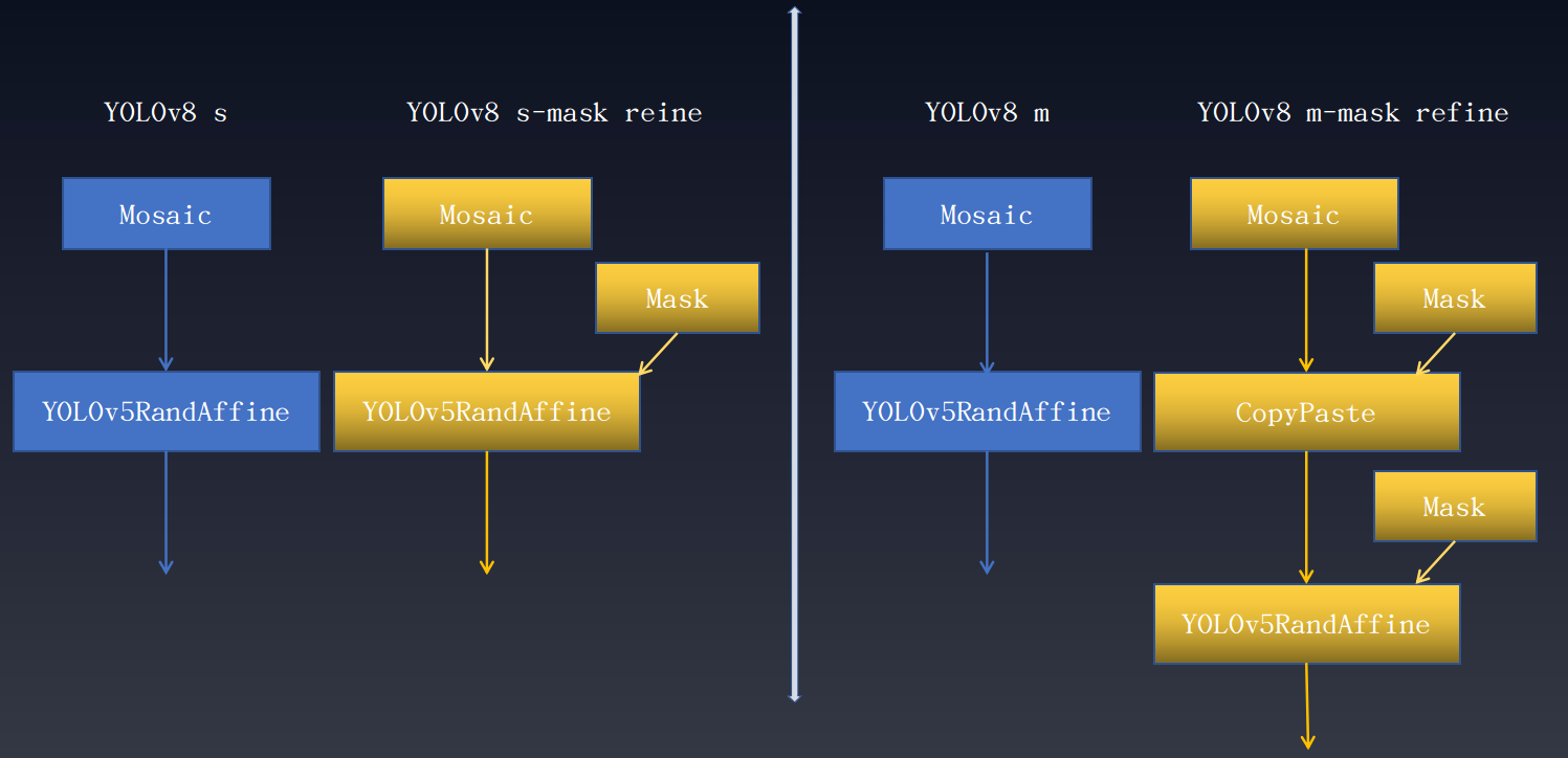
The above-mentioned Mask represents a data augmentation transformation in which instance segmentation annotations play a key role. The application of this technique to other YOLO series has varying degrees of increase.

3 Turn off strong augmentation in the later stage of training to improve detection performance¶

This strategy is proposed for the first time in YOLOX algorithm and can greatly improve the detection performance. The paper points out that Mosaic+MixUp can greatly improve the target detection performance, but the training pictures are far from the real distribution of natural pictures, and Mosaic’s large number of cropping operations will bring many inaccurate label boxes, therefore, YOLOX proposes to turn off the strong enhancement in the last 15 epochs and use the weaker enhancement instead, so that the detector can avoid the influence of inaccurate labeled boxes and complete the final convergence under the data distribution of the natural picture.

This strategy has been applied to most YOLO algorithms. Taking YOLOv8 as an example, its data augmentation pipeline is shown as follows:

However, when to turn off the strong augmentation is a hyper-parameter. If you turn off the strong augmentation too early, it may not give full play to Mosaic and other strong augmentation effects. If you turn off the strong enhancement too late, it will have no gain because it has been overfitted before. This phenomenon can be observed in YOLOv8 experiment

Backbone	Mask Refine	box AP	Epoch of best mAP
YOLOv8-n	No	37.2	500
YOLOv8-n	Yes	37.4 (+0.2)	499
YOLOv8-s	No	44.2	430
YOLOv8-s	Yes	45.1 (+0.9)	460
YOLOv8-m	No	49.8	460
YOLOv8-m	Yes	50.6 (+0.8)	480
YOLOv8-l	No	52.1	460
YOLOv8-l	Yes	53.0 (+0.9)	491
YOLOv8-x	No	52.7	450
YOLOv8-x	Yes	54.0 (+1.3)	460

As can be seen from the above table:

Large models trained on COCO dataset for 500 epochs are prone to overfitting, and disabling strong augmentations such as Mosaic may not be effective in reducing overfitting in such cases.
Using Mask annotations can alleviate overfitting and improve performance

4 Add pure background images to suppress false positives¶

For non-open-world datasets in object detection, both training and testing are conducted on a fixed set of classes, and there is a possibility of producing false positives when applied to images with classes that have not been trained. A common mitigation strategy is to add a certain proportion of pure background images. In most YOLO series, the function of suppressing false positives by adding pure background images is enabled by default. Users only need to set train_dataloader.dataset.filter_cfg.filter_empty_gt to False, indicating that pure background images should not be filtered out during training.

5 Maybe the AdamW works wonders¶

YOLOv5, YOLOv6, YOLOv7 and YOLOv8 all adopt the SGD optimizer, which is strict about parameter settings, while AdamW is on the contrary, which is not so sensitive to learning rate. If user fine-tune a custom-dataset can try to select the AdamW optimizer. We did a simple trial in YOLOX and found that replacing the optimizer with AdamW on the tiny, s, and m scale models all had some improvement.

Backbone	Size	Batch Size	RTMDet-Hyp	Box AP
YOLOX-tiny	416	8xb8	No	32.7
YOLOX-tiny	416	8xb32	Yes	34.3 (+1.6)
YOLOX-s	640	8xb8	No	40.7
YOLOX-s	640	8xb32	Yes	41.9 (+1.2)
YOLOX-m	640	8xb8	No	46.9
YOLOX-m	640	8xb32	Yes	47.5 (+0.6)

More details can be found in configs/yolox/README.md.

6 Consider ignore scenarios to avoid uncertain annotations¶

Take CrowdHuman as an example, a crowded pedestrian detection dataset. Here’s a typical image:

The image is sourced from detectron2 issue. The area marked with a yellow cross indicates the iscrowd label. There are two reasons for this:

This area is not a real person, such as the person on the poster
The area is too crowded to mark

In this scenario, you cannot simply delete such annotations, because once you delete them, it means treating them as background areas during training. However, they are different from the background. Firstly, the people on the posters are very similar to real people, and there are indeed people in crowded areas that are difficult to annotate. If you simply train them as background, it will cause false negatives. The best approach is to treat the crowded area as an ignored region, where any output in this area is directly ignored, with no loss calculated and no model fitting enforced.

MMYOLO quickly and easily verifies the function of ‘iscrowd’ annotation on YOLOv5. The performance is as follows:

Backbone	ignore_iof_thr	box AP50(CrowDHuman Metric)	MR	JI
YOLOv5-s	-1	85.79	48.7	75.33
YOLOv5-s	0.5	86.17	48.8	75.87

ignore_iof_thr set to -1 indicates that the ignored labels are not considered, and it can be seen that the performance is improved to a certain extent, more details can be found in CrowdHuman results. If you encounter similar situations in your custom dataset, it is recommended that you consider using ignore labels to avoid uncertain annotations.

7 Use knowledge distillation¶

Knowledge distillation is a widely used technique that can transfer the performance of a large model to a smaller model, thereby improving the detection performance of the smaller model. Currently, MMYOLO and MMRazor have supported this feature and conducted initial verification on RTMDet.

Model	box AP
RTMDet-tiny	41.0
RTMDet-tiny *	41.8 (+0.8)
RTMDet-s	44.6
RTMDet-s *	45.7 (+1.1)
RTMDet-m	49.3
RTMDet-m *	50.2 (+0.9)
RTMDet-l	51.4
RTMDet-l *	52.3 (+0.9)

* indicates the result of using the large model distillation, more details can be found in Distill RTMDet.

8 Stronger augmentation parameters are used for larger models¶

If you have modified the model based on the default configuration or replaced the backbone network, it is recommended to scale the data augmentation parameters based on the current model size. Generally, larger models require stronger augmentation parameters, otherwise they may not fully leverage the benefits of large models. Conversely, if strong augmentations are applied to small models, it may result in underfitting. Taking RTMDet as an example, we can observe the data augmentation parameters for different model sizes.

random_resize_ratio_range represents the random scaling range of RandomResize, and mosaic_max_cached_images/mixup_max_cached_images represents the number of cached images during Mosaic/MixUp augmentation, which can be used to adjust the strength of augmentation. The YOLO series models all follow the same set of parameter settings principles.

Accelerate training speed¶

1 Enable cudnn_benchmark for single-scale training¶

Most of the input image sizes in the YOLO series algorithms are fixed, which is single-scale training. In this case, you can turn on cudnn_benchmark to accelerate the training speed. This parameter is mainly set for PyTorch’s cuDNN underlying library, and setting this flag can allow the built-in cuDNN to automatically find the most efficient algorithm that is best suited for the current configuration to optimize the running efficiency. If this flag is turned on in multi-scale mode, it will continuously search for the optimal algorithm, which may slow down the training speed instead.

To enable cudnn_benchmark in MMYOLO, you can set env_cfg = dict(cudnn_benchmark=True) in the configuration.

2 Use Mosaic and MixUp with caching¶

If you have applied Mosaic and MixUp in your data augmentation, and after investigating the training bottleneck, it is found that the random image reading is causing the issue, then it is recommended to replace the regular Mosaic and MixUp with the cache-enabled versions proposed in RTMDet.

Data Aug	Use cache	ms/100 imgs
Mosaic	No	87.1
Mosaic	Yes	24.0
MixUp	No	19.3
MixUp	Yes	12.4

Mosaic and MixUp involve mixing multiple images, and their time consumption is K times that of ordinary data augmentation (K is the number of images mixed). For example, in YOLOv5, when doing Mosaic each time, the information of 4 images needs to be reloaded from the hard disk. However, the cached version of Mosaic and MixUp only needs to reload the current image, while the remaining images involved in the mixed augmentation are obtained from the cache queue, greatly improving efficiency by sacrificing a certain amount of memory space.

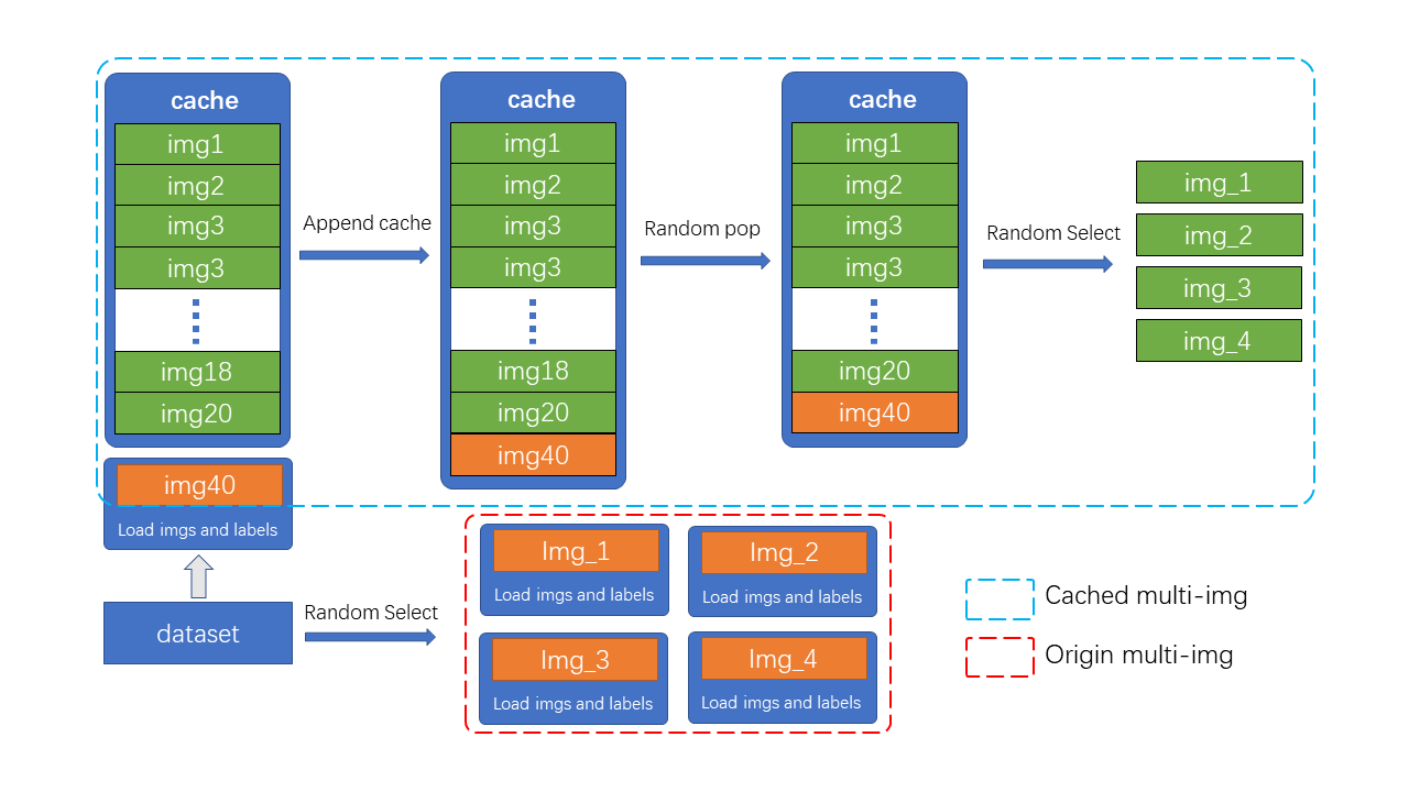
As shown in the figure, N preloaded images and label data are stored in the cache queue. In each training step, only one new image and its label data need to be loaded and updated in the cache queue. (Images in the cache queue can be duplicated, as shown in the figure with img3 appearing twice.) If the length of the cache queue exceeds the preset length, a random image will be popped out. When it is necessary to perform mixed data augmentation, only the required images need to be randomly selected from the cache for concatenation or other processing, without the need to load all images from the hard disk, thus saving image loading time.

Reduce the number of hyperparameter¶

YOLOv5 provides some practical methods for reducing the number of hyperparameter, which are described below.

1 Adaptive loss weighting, reducing one hyperparameter¶

In general, it can be challenging to set hyperparameters specifically for different tasks or categories. YOLOv5 proposes some adaptive methods for scaling loss weights based on the number of classes and the number of detection output layers have been proposed based on practical experience, as shown below:

# scaled based on number of detection layers
loss_cls=dict(
    type='mmdet.CrossEntropyLoss',
    use_sigmoid=True,
    reduction='mean',
    loss_weight=loss_cls_weight *
    (num_classes / 80 * 3 / num_det_layers)),
loss_bbox=dict(
    type='IoULoss',
    iou_mode='ciou',
    bbox_format='xywh',
    eps=1e-7,
    reduction='mean',
    loss_weight=loss_bbox_weight * (3 / num_det_layer
    return_iou=True),
loss_obj=dict(
    type='mmdet.CrossEntropyLoss',
    use_sigmoid=True,
    reduction='mean',
    loss_weight=loss_obj_weight *
    ((img_scale[0] / 640)**2 * 3 / num_det_layers)),

loss_cls can adaptively scale loss_weight based on the custom number of classes and the number of detection layers, loss_bbox can adaptively calculate based on the number of detection layers, and loss_obj can adaptively scale based on the input image size and the number of detection layers. This strategy allows users to avoid setting Loss weight hyperparameters. It should be noted that this is only an empirical principle and not necessarily the optimal setting combination, it should be used as a reference.

2 Adaptive Weight Decay and Loss output values base on Batch Size, reducing two hyperparameters¶

In general,when training on different Batch Size, it is necessary to follow the rule of automatic learning rate scaling. However, validation on various datasets shows that YOLOv5 can achieve good results without scaling the learning rate when changing the Batch Size, and sometimes scaling can even lead to worse results. The reason lies in the technique of Weight Decay and Loss output based on Batch Size adaptation in the code. In YOLOv5, Weight Decay and Loss output values will be scaled based on the total Batch Size being trained. The corresponding code is:

# https://github.com/open-mmlab/mmyolo/blob/dev/mmyolo/engine/optimizers/yolov5_optim_constructor.py#L86
if 'batch_size_per_gpu' in optimizer_cfg:
    batch_size_per_gpu = optimizer_cfg.pop('batch_size_per_gpu')
    # No scaling if total_batch_size is less than
    # base_total_batch_size, otherwise linear scaling.
    total_batch_size = get_world_size() * batch_size_per_gpu
    accumulate = max(
        round(self.base_total_batch_size / total_batch_size), 1)
    scale_factor = total_batch_size * \
        accumulate / self.base_total_batch_size
    if scale_factor != 1:
        weight_decay *= scale_factor
        print_log(f'Scaled weight_decay to {weight_decay}', 'current')

# https://github.com/open-mmlab/mmyolo/blob/dev/mmyolo/models/dense_heads/yolov5_head.py#L635
 _, world_size = get_dist_info()
 return dict(
     loss_cls=loss_cls * batch_size * world_size,
     loss_obj=loss_obj * batch_size * world_size,
     loss_bbox=loss_box * batch_size * world_size)

The weight of Loss varies in different Batch Sizes, and generally, the larger Batch Size means most larger the Loss and gradient. I personally speculate that this can be equivalent to a scenario of linearly increasing learning rate when Batch Size increases. In fact, from the YOLOv5 Study: mAP vs Batch-Size of YOLOv5, it can be found that it is desirable for users to achieve similar performance without modifying other parameters when modifying the Batch Size. The above two strategies are very good training techniques.

Save memory on GPU¶

How to reduce training memory usage is a frequently discussed issue, and there are many techniques involved. The training executor of MMYOLO comes from MMEngine, so you can refer to the MMEngine documentation for how to reduce training memory usage. Currently, MMEngine supports gradient accumulation, gradient checkpointing, and large model training techniques, details of which can be found in the SAVE MEMORY ON GPU.

Testing trick¶

Balance between inference speed and testing accuracy¶

During model performance testing, we generally require a higher mAP, but in practical applications or inference, we want the model to perform faster while maintaining low false positive and false negative rates. In other words, the testing only focuses on mAP while ignoring post-processing and evaluation speed, while in practical applications, a balance between speed and accuracy is pursued. In the YOLO series, it is possible to achieve a balance between speed and accuracy by controlling certain parameters. In this example, we will describe this in detail using YOLOv5.

1 Avoiding multiple class outputs for a single detection box during inference¶

YOLOv5 uses BCE Loss (use_sigmoid=True) during the training of the classification branch. Assuming there are 4 object categories, the number of categories output by the classification branch is 4 instead of 5. Moreover, due to the use of sigmoid instead of softmax prediction, it is possible to predict multiple detection boxes that meet the filtering threshold at a certain position, which means that there may be a situation where one predicted bbox corresponds to multiple predicted labels. This is shown in the figure below:

Generally, when calculating mAP, the filtering threshold is set to 0.001. Due to the non-competitive prediction mode of sigmoid, one box may correspond to multiple labels. This calculation method can increase the recall rate when calculating mAP, but it may not be convenient for practical applications.

One common approach is to increase the filtering threshold. However, if you don’t want to have many false negatives, it is recommended to set the multi_label parameter to False. It is located in the configuration file at mode.test_cfg.multi_label and its default value is True, which allows one detection box to correspond to multiple labels.

2 Simplify test pipeline¶

Note that the test pipeline for YOLOv5 is as follows:

test_pipeline = [
    dict(type='LoadImageFromFile'),
    dict(type='YOLOv5KeepRatioResize', scale=img_scale),
    dict(
        type='LetterResize',
        scale=img_scale,
        allow_scale_up=False,
        pad_val=dict(img=114)),
    dict(type='LoadAnnotations', with_bbox=True, _scope_='mmdet'),
    dict(
        type='mmdet.PackDetInputs',
        meta_keys=('img_id', 'img_path', 'ori_shape', 'img_shape',
                   'scale_factor', 'pad_param'))
]

It uses two different Resizes with different functions, with the aim of improving the mAP value during evaluation. In actual deployment, you can simplify this pipeline as shown below:

test_pipeline = [
    dict(type='LoadImageFromFile'),
    dict(
        type='LetterResize',
        scale=_base_.img_scale,
        allow_scale_up=True,
        use_mini_pad=True),
    dict(type='LoadAnnotations', with_bbox=True),
    dict(
        type='mmdet.PackDetInputs',
        meta_keys=('img_id', 'img_path', 'ori_shape', 'img_shape',
                   'scale_factor', 'pad_param'))
]

In practical applications, YOLOv5 algorithm uses a simplified pipeline with multi_label set to False, score_thr increased to 0.25, and iou_threshold reduced to 0.45. In the YOLOv5 configuration, we provide a set of configuration parameters for detection on the ground, as detailed in yolov5_s-v61_syncbn-detect_8xb16-300e_coco.py.

3 Batch Shape speeds up the testing speed¶

Batch Shape is a testing technique proposed in YOLOv5 that can speed up inference. The idea is to no longer require that all images in the testing process be 640x640, but to test at variable scales, as long as the shapes within the current batch are the same. This approach can reduce additional image pixel padding and speed up the inference process. The specific implementation of Batch Shape can be found in the link. Almost all algorithms in MMYOLO default to enabling the Batch Shape strategy during testing. If users want to disable this feature, you can set val_dataloader.dataset.batch_shapes_cfg=None.

In practical applications, because dynamic shape is not as fast and efficient as fixed shape. Therefore, this strategy is generally not used in real-world scenarios.

TTA improves test accuracy¶

Data augmentation with TTA (Test Time Augmentation) is a versatile trick that can improve the performance of object detection models and is particularly useful in competition scenarios. MMYOLO has already supported TTA, and it can be enabled simply by adding --tta when testing. For more details, please refer to the TTA.