15 minutes to get started with MMYOLO object detection
Object detection task refers to that given a picture, the network predicts all the categories of objects included in the picture and the corresponding boundary boxes
Take the small dataset of cat as an example, you can easily learn MMYOLO object detection in 15 minutes. The whole process consists of the following steps:
In this tutorial, we take YOLOv5-s as an example. For the rest of the YOLO series algorithms, please see the corresponding algorithm configuration folder.
Installation
Assuming you’ve already installed Conda in advance, then install PyTorch using the following commands.
Note
Note: Since this repo uses OpenMMLab 2.0, it is better to create a new conda virtual environment to prevent conflicts with the repo installed in OpenMMLab 1.0.
conda create -n mmyolo python=3.8 -y
conda activate mmyolo
# If you have GPU
conda install pytorch torchvision -c pytorch
# If you only have CPU
# conda install pytorch torchvision cpuonly -c pytorch
Install MMYOLO and dependency libraries using the following commands.
git clone https://github.com/open-mmlab/mmyolo.git
cd mmyolo
pip install -U openmim
mim install -r requirements/mminstall.txt
# Install albumentations
mim install -r requirements/albu.txt
# Install MMYOLO
mim install -v -e .
# "-v" means verbose, or more output
# "-e" means installing a project in editable mode,
# thus any local modifications made to the code will take effect without reinstallation.
For details about how to configure the environment, see Installation and verification.
Dataset
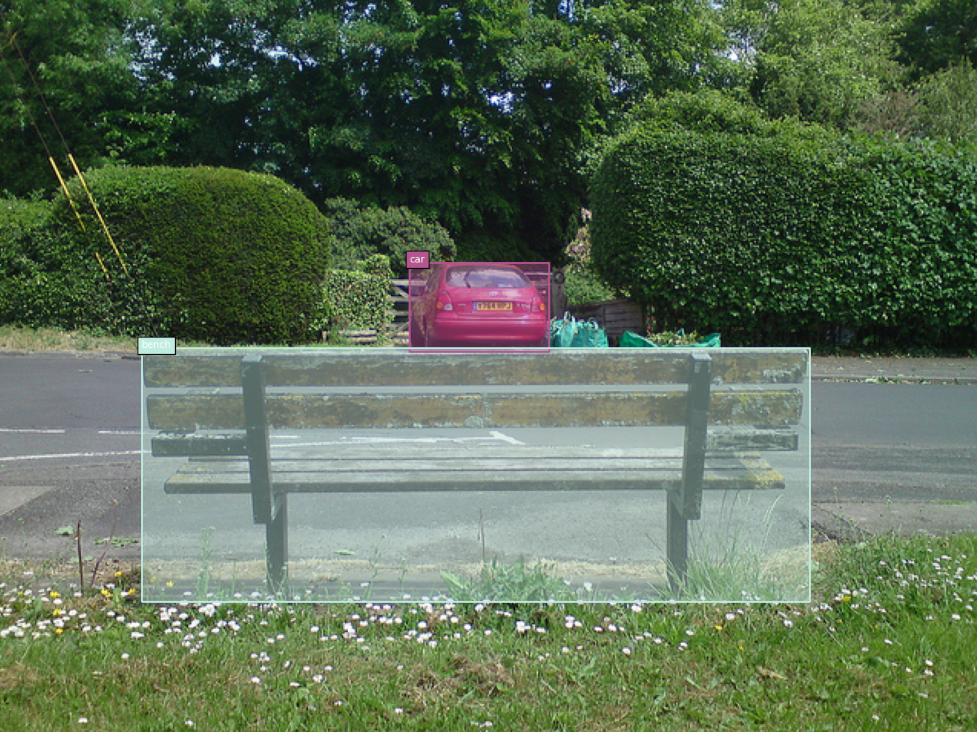
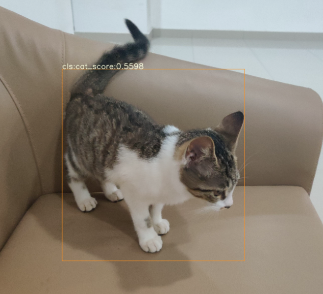
The Cat dataset is a single-category dataset consisting of 144 pictures (the original pictures are provided by @RangeKing, and cleaned by @PeterH0323), which contains the annotation information required for training. The sample image is shown below:

You can download and use it directly by the following command:
python tools/misc/download_dataset.py --dataset-name cat --save-dir ./data/cat --unzip --delete
This dataset is automatically downloaded to the ./data/cat dir with the following directory structure:

The cat dataset is located in the mmyolo project dir, and data/cat/annotations stores annotations in COCO format, and data/cat/images stores all images
Config
Taking YOLOv5 algorithm as an example, considering the limited GPU memory of users, we need to modify some default training parameters to make them run smoothly. The key parameters to be modified are as follows:
YOLOv5 is an Anchor-Based algorithm, and different datasets need to calculate suitable anchors adaptively
The default config uses 8 GPUs with a batch size of 16 per GPU. Now change it to a single GPU with a batch size of 12.
The default training epoch is 300. Change it to 40 epoch
Given the small size of the dataset, we opted to use fixed backbone weights
In principle, the learning rate should be linearly scaled accordingly when the batch size is changed, but actual measurements have found that this is not necessary
Create a yolov5_s-v61_fast_1xb12-40e_cat.py config file in the configs/yolov5 folder (we have provided this config for you to use directly) and copy the following into the config file.
# Inherit and overwrite part of the config based on this config
_base_ = 'yolov5_s-v61_syncbn_fast_8xb16-300e_coco.py'

data_root = './data/cat/' # dataset root
class_name = ('cat', ) # dataset category name
num_classes = len(class_name) # dataset category number
# metainfo is a configuration that must be passed to the dataloader, otherwise it is invalid
# palette is a display color for category at visualization
# The palette length must be greater than or equal to the length of the classes
metainfo = dict(classes=class_name, palette=[(20, 220, 60)])

# Adaptive anchor based on tools/analysis_tools/optimize_anchors.py
anchors = [
    [(68, 69), (154, 91), (143, 162)],  # P3/8
    [(242, 160), (189, 287), (391, 207)],  # P4/16
    [(353, 337), (539, 341), (443, 432)]  # P5/32
]
# Max training 40 epoch
max_epochs = 40
# Set batch size to 12
train_batch_size_per_gpu = 12
# dataloader num workers
train_num_workers = 4

# load COCO pre-trained weight
load_from = 'https://download.openmmlab.com/mmyolo/v0/yolov5/yolov5_s-v61_syncbn_fast_8xb16-300e_coco/yolov5_s-v61_syncbn_fast_8xb16-300e_coco_20220918_084700-86e02187.pth'  # noqa

model = dict(
    # Fixed the weight of the entire backbone without training
    backbone=dict(frozen_stages=4),
    bbox_head=dict(
        head_module=dict(num_classes=num_classes),
        prior_generator=dict(base_sizes=anchors)
    ))

train_dataloader = dict(
    batch_size=train_batch_size_per_gpu,
    num_workers=train_num_workers,
    dataset=dict(
        data_root=data_root,
        metainfo=metainfo,
        # Dataset annotation file of json path
        ann_file='annotations/trainval.json',
        # Dataset prefix
        data_prefix=dict(img='images/')))

val_dataloader = dict(
    dataset=dict(
        metainfo=metainfo,
        data_root=data_root,
        ann_file='annotations/test.json',
        data_prefix=dict(img='images/')))

test_dataloader = val_dataloader

_base_.optim_wrapper.optimizer.batch_size_per_gpu = train_batch_size_per_gpu

val_evaluator = dict(ann_file=data_root + 'annotations/test.json')
test_evaluator = val_evaluator

default_hooks = dict(
    # Save weights every 10 epochs and a maximum of two weights can be saved.
    # The best model is saved automatically during model evaluation
    checkpoint=dict(interval=10, max_keep_ckpts=2, save_best='auto'),
    # The warmup_mim_iter parameter is critical.
    # The default value is 1000 which is not suitable for cat datasets.
    param_scheduler=dict(max_epochs=max_epochs, warmup_mim_iter=10),
    # The log printing interval is 5
    logger=dict(type='LoggerHook', interval=5))
# The evaluation interval is 10
train_cfg = dict(max_epochs=max_epochs, val_interval=10)
The above config is inherited from yolov5_s-v61_syncbn_fast_8xb16-300e_coco.py. According to the characteristics of cat dataset updated data_root, metainfo, train_dataloader, val_dataloader, num_classes and other config.
Training
python tools/train.py configs/yolov5/yolov5_s-v61_fast_1xb12-40e_cat.py
Run the above training command, work_dirs/yolov5_s-v61_fast_1xb12-40e_cat folder will be automatically generated, the checkpoint file and the training config file will be saved in this folder. On a low-end 1660 GPU, the entire training process takes about eight minutes.

The performance on test.json is as follows:
 Average Precision  (AP) @[ IoU=0.50:0.95 | area=   all | maxDets=100 ] = 0.631
 Average Precision  (AP) @[ IoU=0.50      | area=   all | maxDets=100 ] = 0.909
 Average Precision  (AP) @[ IoU=0.75      | area=   all | maxDets=100 ] = 0.747
 Average Precision  (AP) @[ IoU=0.50:0.95 | area= small | maxDets=100 ] = -1.000
 Average Precision  (AP) @[ IoU=0.50:0.95 | area=medium | maxDets=100 ] = -1.000
 Average Precision  (AP) @[ IoU=0.50:0.95 | area= large | maxDets=100 ] = 0.631
 Average Recall     (AR) @[ IoU=0.50:0.95 | area=   all | maxDets=  1 ] = 0.627
 Average Recall     (AR) @[ IoU=0.50:0.95 | area=   all | maxDets= 10 ] = 0.703
 Average Recall     (AR) @[ IoU=0.50:0.95 | area=   all | maxDets=100 ] = 0.703
 Average Recall     (AR) @[ IoU=0.50:0.95 | area= small | maxDets=100 ] = -1.000
 Average Recall     (AR) @[ IoU=0.50:0.95 | area=medium | maxDets=100 ] = -1.000
 Average Recall     (AR) @[ IoU=0.50:0.95 | area= large | maxDets=100 ] = 0.703
The above properties are printed via the COCO API, where -1 indicates that no object exists for the scale. According to the rules defined by COCO, the Cat dataset contains all large sized objects, and there are no small or medium-sized objects.
Some Notes
Two key warnings are printed during training:
You are using
YOLOv5Headwith num_classes == 1. The loss_cls will be 0. This is a normal phenomenon.The model and loaded state dict do not match exactly
Neither of these warnings will have any impact on performance. The first warning is because the num_classes currently trained is 1, the loss of the classification branch is always 0 according to the community of the YOLOv5 algorithm, which is a normal phenomenon. The second warning is because we are currently training in fine-tuning mode, we load the COCO pre-trained weights for 80 classes,
This will lead to the final Head module convolution channel number does not correspond, resulting in this part of the weight can not be loaded, which is also a normal phenomenon.
Training is resumed after the interruption
If you stop training, you can add --resume to the end of the training command and the program will automatically resume training with the latest weights file from work_dirs.
python tools/train.py configs/yolov5/yolov5_s-v61_fast_1xb12-40e_cat.py --resume
Save GPU memory strategy
The above config requires about 3G RAM, so if you don’t have enough, consider turning on mixed-precision training
python tools/train.py configs/yolov5/yolov5_s-v61_fast_1xb12-40e_cat.py --amp
Training visualization
MMYOLO currently supports local, TensorBoard, WandB and other back-end visualization. The default is to use local visualization, and you can switch to WandB and other real-time visualization of various indicators in the training process.
1 WandB
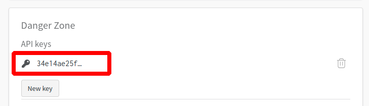
WandB visualization need registered in website, and in the https://wandb.ai/settings for wandb API Keys.
pip install wandb
# After running wandb login, enter the API Keys obtained above, and the login is successful.
wandb login
Add the wandb config at the end of config file we just created: configs/yolov5/yolov5_s-v61_fast_1xb12-40e_cat.py.
visualizer = dict(vis_backends = [dict(type='LocalVisBackend'), dict(type='WandbVisBackend')])
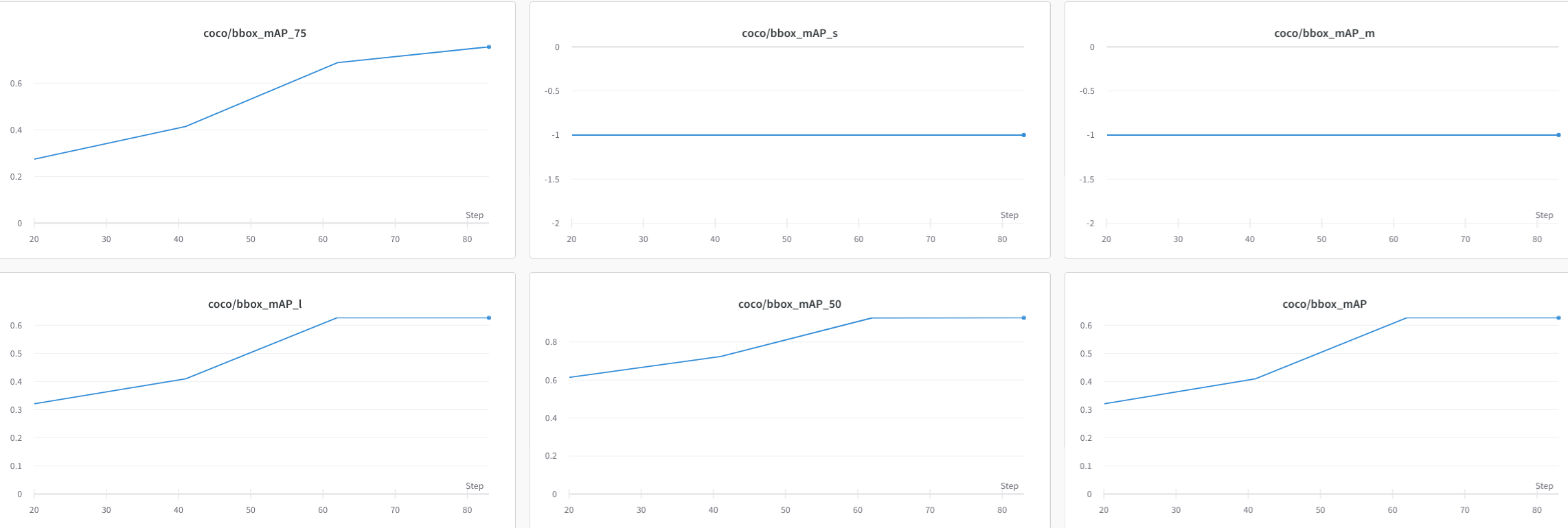
Running the training command and you will see the loss, learning rate, and coco/bbox_mAP visualizations in the link.
python tools/train.py configs/yolov5/yolov5_s-v61_fast_1xb12-40e_cat.py

2 Tensorboard
Install Tensorboard package:
pip install tensorboard
Add the tensorboard config at the end of config file we just created: configs/yolov5/yolov5_s-v61_fast_1xb12-40e_cat.py.
visualizer = dict(vis_backends=[dict(type='LocalVisBackend'),dict(type='TensorboardVisBackend')])
After re-running the training command, Tensorboard file will be generated in the visualization folder work_dirs/yolov5_s-v61_fast_1xb12-40e_cat/{timestamp}/vis_data.
We can use Tensorboard to view the loss, learning rate, and coco/bbox_mAP visualizations from a web link by running the following command:
tensorboard --logdir=work_dirs/yolov5_s-v61_fast_1xb12-40e_cat
Testing
python tools/test.py configs/yolov5/yolov5_s-v61_fast_1xb12-40e_cat.py \
                     work_dirs/yolov5_s-v61_fast_1xb12-40e_cat/epoch_40.pth \
                     --show-dir show_results
Run the above test command, you can not only get the AP performance printed in the Training section, You can also automatically save the result images to the work_dirs/yolov5_s-v61_fast_1xb12-40e_cat/{timestamp}/show_results folder. Below is one of the result images, the left image is the actual annotation, and the right image is the inference result of the model.

You can also visualize model inference results in a browser window if you use ‘WandbVisBackend’ or ‘TensorboardVisBackend’.
Feature map visualization
MMYOLO provides visualization scripts for feature map to analyze the current model training. Please refer to Feature Map Visualization
Due to the bias of direct visualization of test_pipeline, we need to modify the test_pipeline of configs/yolov5/yolov5_s-v61_syncbn_8xb16-300e_coco.py
test_pipeline = [
    dict(
        type='LoadImageFromFile',
        backend_args=_base_.backend_args),
    dict(type='YOLOv5KeepRatioResize', scale=img_scale),
    dict(
        type='LetterResize',
        scale=img_scale,
        allow_scale_up=False,
        pad_val=dict(img=114)),
    dict(type='LoadAnnotations', with_bbox=True, _scope_='mmdet'),
    dict(
        type='mmdet.PackDetInputs',
        meta_keys=('img_id', 'img_path', 'ori_shape', 'img_shape',
                   'scale_factor', 'pad_param'))
]
to the following config:
test_pipeline = [
    dict(
        type='LoadImageFromFile',
        backend_args=_base_.backend_args),
    dict(type='mmdet.Resize', scale=img_scale, keep_ratio=False), # modify the LetterResize to mmdet.Resize
    dict(type='LoadAnnotations', with_bbox=True, _scope_='mmdet'),
    dict(
        type='mmdet.PackDetInputs',
        meta_keys=('img_id', 'img_path', 'ori_shape', 'img_shape',
                   'scale_factor'))
]
Let’s choose the data/cat/images/IMG_20221020_112705.jpg image as an example to visualize the output feature maps of YOLOv5 backbone and neck layers.
1. Visualize the three channels of YOLOv5 backbone
python demo/featmap_vis_demo.py data/cat/images/IMG_20221020_112705.jpg \
                                configs/yolov5/yolov5_s-v61_fast_1xb12-40e_cat.py \
                                work_dirs/yolov5_s-v61_fast_1xb12-40e_cat/epoch_40.pth \
                                --target-layers backbone \
                                --channel-reduction squeeze_mean
The result will be saved to the output folder in current path. Three output feature maps plotted in the above figure correspond to small, medium and large output feature maps. As the backbone of this training is not actually involved in training, it can be seen from the above figure that the big object cat is predicted on the small feature map, which is in line with the idea of hierarchical detection of object detection.
2. Visualize the three channels of YOLOv5 neck
python demo/featmap_vis_demo.py data/cat/images/IMG_20221020_112705.jpg \
                                configs/yolov5/yolov5_s-v61_fast_1xb12-40e_cat.py \
                                work_dirs/yolov5_s-v61_fast_1xb12-40e_cat/epoch_40.pth \
                                --target-layers neck \
                                --channel-reduction squeeze_mean

As can be seen from the above figure, because neck is involved in training, and we also reset anchor, the three output feature maps are forced to simulate the same scale object, resulting in the three output maps of neck are similar, which destroys the original pre-training distribution of backbone. At the same time, it can also be seen that 40 epochs are not enough to train the above dataset, and the feature maps do not perform well.
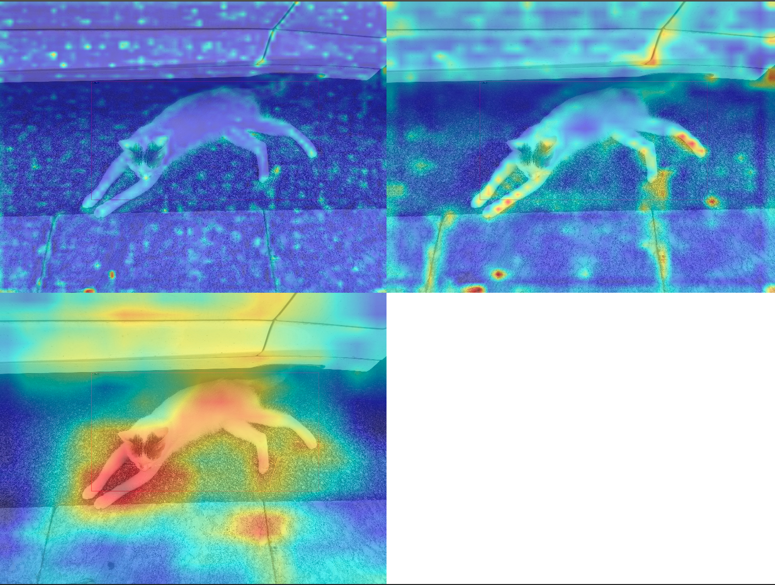
3. Grad-Based CAM visualization
Based on the above feature map visualization, we can analyze Grad CAM at the feature layer of bbox level.
Install grad-cam package:
pip install "grad-cam"
(a) View Grad CAM of the minimum output feature map of the neck
python demo/boxam_vis_demo.py data/cat/images/IMG_20221020_112705.jpg \
                              configs/yolov5/yolov5_s-v61_fast_1xb12-40e_cat.py \
                              work_dirs/yolov5_s-v61_fast_1xb12-40e_cat/epoch_40.pth \
                              --target-layer neck.out_layers[2]

(b) View Grad CAM of the medium output feature map of the neck
python demo/boxam_vis_demo.py data/cat/images/IMG_20221020_112705.jpg \
                              configs/yolov5/yolov5_s-v61_fast_1xb12-40e_cat.py \
                              work_dirs/yolov5_s-v61_fast_1xb12-40e_cat/epoch_40.pth \
                              --target-layer neck.out_layers[1]

(c) View Grad CAM of the maximum output feature map of the neck
python demo/boxam_vis_demo.py data/cat/images/IMG_20221020_112705.jpg \
                              configs/yolov5/yolov5_s-v61_fast_1xb12-40e_cat.py \
                              work_dirs/yolov5_s-v61_fast_1xb12-40e_cat/epoch_40.pth \
                              --target-layer neck.out_layers[0]

EasyDeploy deployment
Here we’ll use MMYOLO’s EasyDeploy to demonstrate the transformation deployment and basic inference of model.
First you need to follow EasyDeploy’s basic documentation controls own equipment installed for each library.
pip install onnx
pip install onnx-simplifier # Install if you want to use simplify
pip install tensorrt        # If you have GPU environment and need to output TensorRT model you need to continue execution
Once installed, you can use the following command to transform and deploy the trained model on the cat dataset with one click. The current ONNX version is 1.13.0 and TensorRT version is 8.5.3.1, so keep the --opset value of 11. The remaining parameters need to be adjusted according to the config used. Here we export the CPU version of ONNX with the --backend set to 1.
python projects/easydeploy/tools/export.py \
	configs/yolov5/yolov5_s-v61_fast_1xb12-40e_cat.py \
	work_dirs/yolov5_s-v61_fast_1xb12-40e_cat/epoch_40.pth \
	--work-dir work_dirs/yolov5_s-v61_fast_1xb12-40e_cat \
    --img-size 640 640 \
    --batch 1 \
    --device cpu \
    --simplify \
	--opset 11 \
	--backend 1 \
	--pre-topk 1000 \
	--keep-topk 100 \
	--iou-threshold 0.65 \
	--score-threshold 0.25
On success, you will get the converted ONNX model under work-dir, which is named end2end.onnx by default.
Let’s use end2end.onnx model to perform a basic image inference:
python projects/easydeploy/tools/image-demo.py \
    data/cat/images/IMG_20210728_205312.jpg \
    configs/yolov5/yolov5_s-v61_fast_1xb12-40e_cat.py \
    work_dirs/yolov5_s-v61_fast_1xb12-40e_cat/end2end.onnx \
    --device cpu
After successful inference, the result image will be generated in the output folder of the default MMYOLO root directory. If you want to see the result without saving it, you can add --show to the end of the above command. For convenience, the following is the generated result.
Let’s go on to convert the engine file for TensorRT, because TensorRT needs to be specific to the current environment and deployment version, so make sure to export the parameters, here we export the TensorRT8 file, the --backend is 2.
python projects/easydeploy/tools/export.py \
    configs/yolov5/yolov5_s-v61_fast_1xb12-40e_cat.py \
    work_dirs/yolov5_s-v61_fast_1xb12-40e_cat/epoch_40.pth \
    --work-dir work_dirs/yolov5_s-v61_fast_1xb12-40e_cat \
    --img-size 640 640 \
    --batch 1 \
    --device cuda:0 \
    --simplify \
    --opset 11 \
    --backend 2 \
    --pre-topk 1000 \
    --keep-topk 100 \
    --iou-threshold 0.65 \
    --score-threshold 0.25
The resulting end2end.onnx is the ONNX file for the TensorRT8 deployment, which we will use to complete the TensorRT engine transformation.
python projects/easydeploy/tools/build_engine.py \
    work_dirs/yolov5_s-v61_fast_1xb12-40e_cat/end2end.onnx \
    --img-size 640 640 \
    --device cuda:0
Successful execution will generate the end2end.engine file under work-dir:
work_dirs/yolov5_s-v61_fast_1xb12-40e_cat
├── 202302XX_XXXXXX
│   ├── 202302XX_XXXXXX.log
│   └── vis_data
│       ├── 202302XX_XXXXXX.json
│       ├── config.py
│       └── scalars.json
├── best_coco
│   └── bbox_mAP_epoch_40.pth
├── end2end.engine
├── end2end.onnx
├── epoch_30.pth
├── epoch_40.pth
├── last_checkpoint
└── yolov5_s-v61_fast_1xb12-40e_cat.py
Let’s continue use image-demo.py for image inference:
python projects/easydeploy/tools/image-demo.py \
    data/cat/images/IMG_20210728_205312.jpg \
    configs/yolov5/yolov5_s-v61_fast_1xb12-40e_cat.py \
    work_dirs/yolov5_s-v61_fast_1xb12-40e_cat/end2end.engine \
    --device cuda:0
Here we choose to save the inference results under output instead of displaying them directly. The following shows the inference results.

This completes the transformation deployment of the trained model and checks the inference results. This is the end of the tutorial.
The full content above can be viewed in 15_minutes_object_detection.ipynb. If you encounter problems during training or testing, please check the common troubleshooting steps first and feel free to open an issue if you still can’t solve it.