A benchmark for ionogram real-time object detection based on MMYOLO

Dataset

Digital ionogram is the most important way to obtain real-time ionospheric information. Ionospheric structure detection is of great research significance for accurate extraction of ionospheric key parameters.

This study utilize 4311 ionograms with different seasons obtained by the Chinese Academy of Sciences in Hainan, Wuhan, and Huailai to establish a dataset. The six structures, including Layer E, Es-l, Es-c, F1, F2, and Spread F are manually annotated using labelme. Dataset Download

Preview of annotated images

1. Dataset prepration

After downloading the data, put it in the root directory of the MMYOLO repository, and use unzip test.zip (for Linux) to unzip it to the current folder. The structure of the unzipped folder is as follows:

Iono4311/
├── images
|      ├── 20130401005200.png
|      └── ...
└── labels
       ├── 20130401005200.json
       └── ...

The images directory contains input images，while the labels directory contains annotation files generated by labelme.

2. Convert the dataset into COCO format

Use the script tools/dataset_converters/labelme2coco.py to convert labelme labels to COCO labels.

python tools/dataset_converters/labelme2coco.py --img-dir ./Iono4311/images \
                                                --labels-dir ./Iono4311/labels \
                                                --out ./Iono4311/annotations/annotations_all.json

3. Check the converted COCO labels

To confirm that the conversion process went successfully, use the following command to display the COCO labels on the images.

python tools/analysis_tools/browse_coco_json.py --img-dir ./Iono4311/images \
                                                --ann-file ./Iono4311/annotations/annotations_all.json

4. Divide dataset into training set, validation set and test set

Set 70% of the images in the dataset as the training set, 15% as the validation set, and 15% as the test set.

python tools/misc/coco_split.py --json ./Iono4311/annotations/annotations_all.json \
                                --out-dir ./Iono4311/annotations \
                                --ratios 0.7 0.15 0.15 \
                                --shuffle \
                                --seed 14

The file tree after division is as follows:

Iono4311/
├── annotations
│   ├── annotations_all.json
│   ├── class_with_id.txt
│   ├── test.json
│   ├── train.json
│   └── val.json
├── classes_with_id.txt
├── images
├── labels
├── test_images
├── train_images
└── val_images

Config files

The configuration files are stored in the directory /projects/misc/ionogram_detection/.

1. Dataset analysis

To perform a dataset analysis, a sample of 200 images from the dataset can be analyzed using the tools/analysis_tools/dataset_analysis.py script.

python tools/analysis_tools/dataset_analysis.py projects/misc/ionogram_detection/yolov5/yolov5_s-v61_fast_1xb96-100e_ionogram.py \
                                                --out-dir output

Part of the output is as follows:

The information obtained is as follows:
+------------------------------+
| Information of dataset class |
+---------------+--------------+
| Class name    | Bbox num     |
+---------------+--------------+
| E             | 98           |
| Es-l          | 27           |
| Es-c          | 46           |
| F1            | 100          |
| F2            | 194          |
| Spread-F      | 6            |
+---------------+--------------+

This indicates that the distribution of categories in the dataset is unbalanced.

Statistics of object sizes for each category

According to the statistics, small objects are predominant in the E, Es-l, Es-c, and F1 categories, while medium-sized objects are more common in the F2 and Spread F categories.

2. Visualization of the data processing part in the config

Taking YOLOv5-s as an example, according to the train_pipeline in the config file, the data augmentation strategies used during training include：

• Mosaic augmentation

• Random affine

• Albumentations (include various digital image processing methods)

• HSV augmentation

• Random affine

Use the ‘pipeline’ mode of the script tools/analysis_tools/browse_dataset.py to obtains all intermediate images in the data pipeline.

python tools/analysis_tools/browse_dataset.py projects/misc/ionogram_detection/yolov5/yolov5_s-v61_fast_1xb96-100e_ionogram.py \
                                              -m pipeline \
                                              --out-dir output

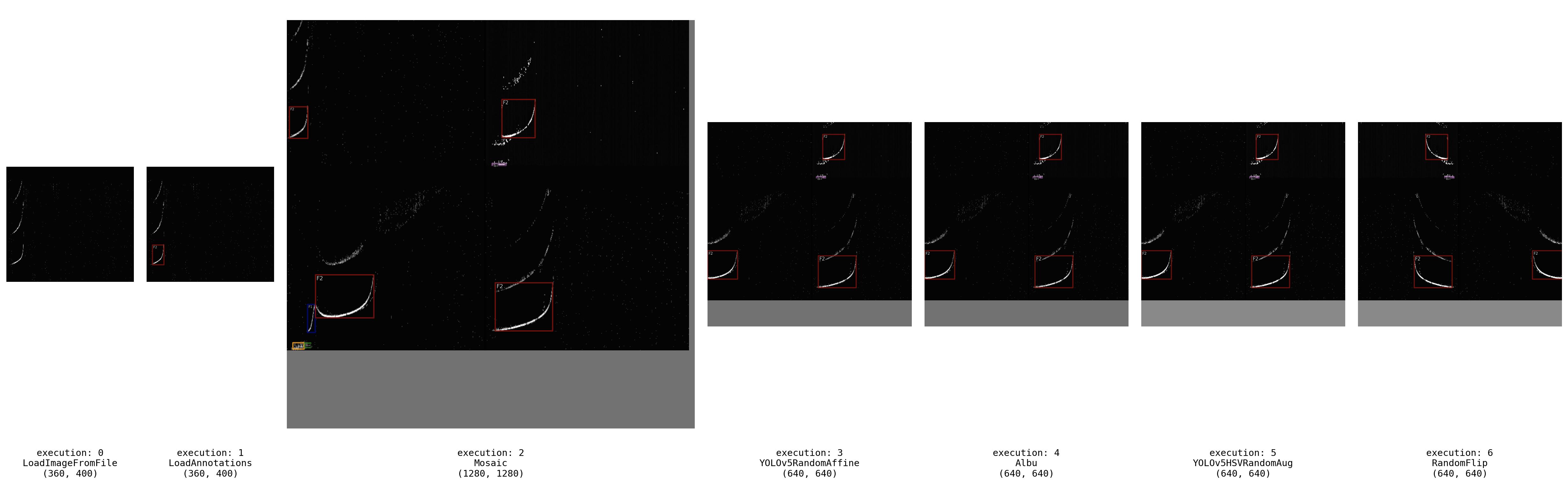
Visualization for intermediate images in the data pipeline

3. Optimize anchor size

Use the script tools/analysis_tools/optimize_anchors.py to obtain prior anchor box sizes suitable for the dataset.

python tools/analysis_tools/optimize_anchors.py projects/misc/ionogram_detection/yolov5/yolov5_s-v61_fast_1xb96-100e_ionogram.py \
                                                --algorithm v5-k-means \
                                                --input-shape 640 640 \
                                                --prior-match-thr 4.0 \
                                                --out-dir work_dirs/dataset_analysis_5_s

4. Model complexity analysis

With the config file, the parameters and FLOPs can be calculated by the script tools/analysis_tools/get_flops.py. Take yolov5-s as an example:

python tools/analysis_tools/get_flops.py projects/misc/ionogram_detection/yolov5/yolov5_s-v61_fast_1xb96-100e_ionogram.py

The following output indicates that the model has 7.947G FLOPs with the input shape (640, 640), and a total of 7.036M learnable parameters.

==============================
Input shape: torch.Size([640, 640])
Model Flops: 7.947G
Model Parameters: 7.036M
==============================

Train and test

1. Train

Training visualization: By following the tutorial of Annotation-to-deployment workflow for custom dataset, this example uses wandb to visulize training.

Debug tricks: During the process of debugging code, sometimes it is necessary to train for several epochs, such as debugging the validation process or checking whether the checkpoint saving meets expectations. For datasets inherited from BaseDataset (such as YOLOv5CocoDataset in this example), setting indices in the dataset field can specify the number of samples per epoch to reduce the iteration time.

train_dataloader = dict(
    batch_size=train_batch_size_per_gpu,
    num_workers=train_num_workers,
    dataset=dict(
        _delete_=True,
        type='RepeatDataset',
        times=1,
        dataset=dict(
            type=_base_.dataset_type,
            indices=200,  # set indices=200，represent every epoch only iterator 200 samples
            data_root=data_root,
            metainfo=metainfo,
            ann_file=train_ann_file,
            data_prefix=dict(img=train_data_prefix),
            filter_cfg=dict(filter_empty_gt=False, min_size=32),
            pipeline=_base_.train_pipeline)))

Start training：

python tools/train.py projects/misc/ionogram_detection/yolov5/yolov5_s-v61_fast_1xb96-100e_ionogram.py

2. Test

Specify the path of the config file and the model to start the test:

python tools/test.py projects/misc/ionogram_detection/yolov5/yolov5_s-v61_fast_1xb96-100e_ionogram.py \
                     work_dirs/yolov5_s-v61_fast_1xb96-100e_ionogram/xxx

Experiments and results

Choose a suitable batch size

• Often, the batch size governs the training speed, and the ideal batch size will be the largest batch size supported by the available hardware.

• If the video memory is not yet fully utilized, doubling the batch size should result in a corresponding doubling (or close to doubling) of the training throughput. This is equivalent to maintaining a constant (or nearly constant) time per step as the batch size increases.

• Automatic Mixed Precision (AMP) is a technique to accelerate the training with minimal loss in accuracy. To enable AMP training, add --amp to the end of the training command.

Hardware information:

• GPU：V100 with 32GB memory

• CPU：10-core CPU with 40GB memory

Results：

Model	Epoch(best)	AMP	Batchsize	Num workers	Memory Allocated	Training Time	Val mAP
YOLOv5-s	100(82)	False	32	6	35.07%	54 min	0.575
YOLOv5-s	100(96)	True	32	6	24.93%	49 min	0.578
YOLOv5-s	100(100)	False	96	6	96.64%	48 min	0.571
YOLOv5-s	100(100)	True	96	6	54.66%	37 min	0.575
YOLOv5-s	100(90)	True	144	6	77.06%	39 min	0.573
YOLOv5-s	200(148)	True	96	6	54.66%	72 min	0.575
YOLOv5-s	200(188)	True	96	8	54.66%	67 min	0.576

The proportion of data loading time to the total time of each step.

Based on the results above, we can conclude that

• AMP has little impact on the accuracy of the model, but can significantly reduce memory usage while training.

• Increasing batch size by three times does not reduce the training time by a corresponding factor of three. According to the data_time recorded during training, the larger the batch size, the larger the data_time, indicating that data loading has become the bottleneck limiting the training speed. Increasing num_workers, the number of processes used to load data, can accelerate the training speed.

Ablation studies

In order to obtain a training pipeline applicable to the dataset, the following ablation studies with the YOLOv5-s model as an example are performed.

Data augmentation

Aug Method	config	config	config	config	config
Mosaic		√	√	√	√
Affine			√	√	√
Albu				√	√
HSV				√	√
Flip					√
Val mAP	0.507	0.550	0.572	0.567	0.575

The results indicate that mosaic augmentation and random affine transformation can significantly improve the performance on the validation set.

Using pre-trained models

If you prefer not to use pre-trained weights, you can simply set load_from = None in the config file. For experiments that do not use pre-trained weights, it is recommended to increase the base learning rate by a factor of four and extend the number of training epochs to 200 to ensure adequate model training.

Model	Epoch(best)	FLOPs(G)	Params(M)	Pretrain	Val mAP	Config
YOLOv5-s	100(82)	7.95	7.04	Coco	0.575	config
YOLOv5-s	200(145)	7.95	7.04	None	0.565	config
YOLOv6-s	100(54)	24.2	18.84	Coco	0.584	config
YOLOv6-s	200(188)	24.2	18.84	None	0.557	config

Comparison of loss reduction during training

The loss reduction curve shows that when using pre-trained weights, the loss decreases faster. It can be seen that even using models pre-trained on natural image datasets can accelerate model convergence when fine-tuned on radar image datasets.

Benchmark for ionogram object detection

Model	epoch(best)	FLOPs(G)	Params(M)	pretrain	val mAP	test mAP	Config	Log
YOLOv5-s	100(82)	7.95	7.04	Coco	0.575	0.584	config	log
YOLOv5-m	100(70)	24.05	20.89	Coco	0.587	0.586	config	log
YOLOv6-s	100(54)	24.2	18.84	Coco	0.584	0.594	config	log
YOLOv6-m	100(76)	37.08	44.42	Coco	0.590	0.590	config	log
YOLOv6-l	100(76)	71.33	58.47	Coco	0.605	0.597	config	log
YOLOv7-tiny	100(78)	6.57	6.02	Coco	0.549	0.568	config	log
YOLOv7-x	100(58)	94.27	70.85	Coco	0.602	0.595	config	log
rtmdet-tiny	100(100)	8.03	4.88	Coco	0.582	0.589	config	log
rtmdet-s	100(92)	14.76	8.86	Coco	0.588	0.585	config	log